Extracting roadway vertical alignment from USGS LiDAR point cloud data using an Artificial Neural Network based method
Abstract
Vertical grades and vertical curvature significantly influence traffic safety. However, obtaining accurate and large-scale data on roadway vertical alignment remains a major challenge. This paper presents a cost-effective and efficient method for estimating roadway vertical alignment using publicly available aerial LiDAR data provided by the United States Geological Survey. An Artificial Neural Network (ANN) model was proposed to predict whether a LiDAR point belongs to a vertical curve or a tangent segment. Due to the limited availability of actual roadway vertical alignment data and the substantial data requirements of machine learning models, a synthetic training dataset was generated by systematically varying road grades and segment lengths to represent realistic combinations of tangents, crest and sag curves. This approach ensured that the model was exposed to a wide range of geometric configurations and allowed it to learn generalized relationships between vertical alignment features and their corresponding geometric parameters. The model was then independently evaluated by comparing the vertical alignment estimated from the extracted aerial LiDAR data for two-lane two-way rural roadways, Route 152 in New Jersey and Route 299 in California, with their corresponding actual vertical alignment data. In addition, a case study was conducted on another rural two-lane highway in which the model was used to compute safe speeds for each roadway segment. The resulting speeds were then compared with the posted speed limits along the corridor. The satisfactory estimation results of this study indicate that the proposed approach can be used for conducting large-scale analyses to estimate vertical alignment using publicly available LiDAR data.
1. Introduction
Roadway vertical alignment consists of grades connected by parabolic curves. Road elevation data are crucial in traffic safety analysis, roadway geometric design, fuel consumption estimation, and highway capacity analysis. Prior studies indicated that crash rates are notably higher on steep grade sections compared to level sections (Glennon, 1987; Yu & Abdel-Aty, 2014). Hamdar et al. (2016) highlighted that driver behaviour is highly influenced by the challenges posed due to the changes in roadway geometric alignment. For instance, abrupt grade changes at crest curves can significantly restrict a driver's line of sight, adversely impacting available stopping sight distance and overall roadway safety. Vertical grades and curvature directly influence sight distance, operating speed, driver workload, and vehicle dynamics, making them central to both geometric design and crash prediction. The American Association of State Highway and Transportation Officials (AASHTO) and the Federal Highway Administration (FHWA) emphasize the role of grades and crest–sag curvature in determining safe stopping distances, speed consistency, and sight limitations on vertical curves (Donnell et al., 2018). Several empirical studies further support this, showing that combinations of horizontal–vertical curvature and steep grades significantly elevate crash risk and reduce speed harmony, particularly on rural two-lane highways (Elvik & Haugvik, 2023;Ryan et al., 2022; Bauer & Harwood, 2013; Papadimitriou et al., 2019; Kar et al., 2024).
Road elevation profiles allow engineers to accurately identify steep grades that pose operational risks, particularly for heavy vehicles, assisting in targeted design interventions like crawler lanes or escape ramps. Moreover, accurate knowledge of road profiles supports safety analysis by helping identify segments with restricted visibility and elevated crash risk, enabling proactive measures such as advisory signage, speed limit adjustments, or geometric redesign. Beyond safety, vertical alignment also governs aspects such as drainage design, fuel consumption, ride comfort, and infrastructure maintenance, while precise elevation modelling facilitates 3D roadway coordination and driver visibility studies (FHWA, 2019).
Moreover, recent flood events in the US underscore the value of roadway elevation profiles in identifying flood-prone segments. Heavy rains in San Antonio and the Tri-State region in the US flooded roadways in 2025, causing fatalities and roadway closures (WTOP News, 2025; MySanAntonio, 2025; National Public Radio, 2025). Accurate vertical alignment extraction, including identification of depressed grades and shallow slopes, can reveal areas prone to ponding or runoff overflow. Integrating these profiles into drainage planning helps agencies implement effective mitigation, such as regrading, culverts, or raised embankments, to improve flood resilience.
Despite its importance, vertical alignment data remain difficult and expensive to obtain at scale. Historically, such information has resided within engineering plans and profile sheets, many of which predate digital storage and are available only in scanned or paper formats. Modern survey techniques such as Global Positioning System (GPS), Global Navigation Satellite System (GNSS), and mobile light detection and ranging (LiDAR) can yield highly precise 3-D elevation data, yet they require specialized survey vehicles, extensive field operations, and substantial financial resources, limiting their use to select corridors (Gargoum & El Basyouny, 2019). Moreover, unlike horizontal alignment, which is traceable through open geospatial databases or aerial imagery, vertical profiles cannot be easily inferred without access to elevation data, making large-scale network coverage a major challenge. This challenge is even more pronounced for older routes, where profile information may be either unavailable or outdated. As a result, estimating the parameters of roadway vertical alignment becomes essential.
Advances in remote sensing and open-access LiDAR now offer a practical solution. The U.S. Geological Survey’s 3D Elevation Program (3DEP) provides nationwide LiDAR coverage with point clouds and digital elevation models available through The National Map, enabling researchers to derive elevation and slope information for most US roads at minimal cost (USGS, 2025). Previous research demonstrates the potential of LiDAR for automated roadway geometry extraction and safety analysis (Yang & Das, 2024; Gargoum & El Basyouny, 2019; Wang et al., 2025). Yet processing large datasets, filtering roadway points, and classifying tangent versus curved segments still require robust analytical approaches.
Various datasets, such as the National Elevation Dataset from the US Geological Survey (USGS NED) (Gesch et al., 2014), Global Digital Elevation Model (GDEM) (Tachikawa et al., 2011), and LiDAR (Reutebuch et al., 2005) elevation datasets are readily available. The 3DEP from the USGS, which employs LiDAR point cloud data, has gathered extensive three-dimensional data across the US. This dataset contains over 12 trillion LiDAR point cloud records, encompassing data from more than 1,254 projects across the country (USGS, 2025).
Various techniques are available for collecting road elevation data, such as GPS, Enhanced GNSS, Inertial Navigation Systems (INS) coupled with GNSS, LiDAR (Baass & Vouland, 2005; Easa & Wang, 2010;Di Mascio et al., 2012; Higuera de Frutos & Castro, 2017; Gargoum et al., 2018; Liu et al., 2018; Zhou et al., 2021; Shams et al., 2023; Holgado-Barco et al., 2014;Yang & Das, 2024), as discussed next in the literature review section. However, these methods may not be feasible due to the cost and effort required for their implementation, especially on a larger scale.
Therefore, there is a need for estimating road elevation data indirectly from available sources, as done for road horizontal alignment (Anil & Natarajan, 2010; Easa et al., 2007;Imran et al., 2006; Yun & Sung, 2005; Xu & Wei, 2016; Bartin et al., 2019; Bartin et al., 2022; Bartin et al., 2021; Bartin et al., 2023; Findley et al., 2012; Luo et al., 2018). However, this topic has not been as extensively explored in the literature. Although various elevation data sources are available, there is a notable absence of methods for extracting roadway vertical alignment using these resources. The ones that use LiDAR data do not rely on replicable methods. In practice, many LiDAR-based studies rely on mobile mapping systems that are not freely available and are often limited to project-specific deployments. The need for advanced survey vehicles raises costs and lengthens data-collection and post-processing, which constrains scalability.
To that end, the objective of this paper is to develop an Artificial Neural Network (ANN) based approach that can accurately, quickly, and affordably extract roadway vertical alignment information and determine its geometric properties using publicly available LiDAR data in the USGS repository (USGS, 2025). However, because the ANN model requires large datasets of known vertical alignment data for training, and such data are not readily available at a large scale, the model was trained and tested using synthetically generated road vertical data. Once trained, the model was able to classify LiDAR points on a roadway as either part of a grade or a vertical curve, considering the surrounding LiDAR points. The developed ANN model was independently evaluated using the actual vertical data of Route 152, a state highway in NJ, and Route 299, a state highway in CA. Also, a case study was conducted on Route 83, a rural two-lane highway in NJ, where the model was applied to regenerate the speed profile.
2. Literature Review
Extracting roadway alignment has been the focus of numerous studies over the years, yet horizontal alignment has been the primary focus alignment (Anil & Natarajan, 2010; Easa et al., 2007;Imran et al., 2006; Yun & Sung, 2005; Xu & Wei, 2016; Bartin et al., 2019; Bartin et al., 2022; Bartin et al., 2021; Bartin et al., 2023; Findley et al., 2012; Luo et al., 2018) Various data sources were utilized for extracting roadway horizontal alignment, ranging from satellite images (Anil & Natarajan, 2010; Easa et al., 2007), GPS data (Imran et al., 2006; Yun & Sung, 2005), Geographic Information System (GIS) maps (Xu & Wei, 2016); (Bartin et al., 2019; Bartin et al., 2022; Bartin et al., 2021; Bartin et al., 2023), and mobile LiDAR mapping (Findley et al., 2012; Luo et al., 2018).
A limited number of studies focused on developing comprehensive and automated methods for extracting roadway vertical alignment. For example, Baass & Vouland, (2005) conducted a study on reconstructing vertical alignment using GPS data sources. They applied the rate of slope change between points to distinguish parabolic curves from the tangents of the vertical alignment. Initially, they used least squares approximation to fit tangents, followed by an iterative process to determine the vertical curves using least square approximations. The process required an initial value for the length of the vertical curve, which was obtained from the previously calculated tangent sections' initial and final grades. They validated the method by comparing it with exact design data and real GPS profile data from Quebec highways. To assess accuracy, they calculated the vertical distance from GPS source points and compared it to the result obtained from calculated alignments. The estimated average error was 15 cm, with a maximum error of 1.5 meters. While they applied some form of filtering to the GNSS data to address irregularities, specific details were not provided. It was acknowledged that factoring in device error would be necessary to measure the absolute error of the procedure.
Easa & Wang (2010) introduced an optimization model aimed at determining the parameters of continuous vertical alignments using GPS data. This model included multiple parabolic vertical curves and aimed to ideally fit the highway profile data through the application of the least squares method. The optimization process operated in two stages: single-curve optimization and multiple-curve optimization. Single-curve optimization employed estimated tangent parameters, derived from the controlling points defined by the operator, to approximate the length of each vertical curve. Conversely, multiple-curve optimization was applied to deduce the globally optimal parameters for both tangents and vertical curves. The model was evaluated using actual data from a 1,700-meter segment of a highway's vertical alignment. To validate the model's accuracy, the study compared the original altitude values with estimated altitudes. The average error observed was 3.8 centimeters.
Di Mascio et al. (2012) utilized a GNSS receiver mounted on a vehicle. They employed the least-squares optimization principle to identify vertical curves and lines that represent the section of the road considered with the respective mobile base. The vertical curves were examined as circular components. As a final step, they fine-tuned the results of their method using the vertical curvature profile. Higuera de Frutos & Castro (2017) developed an algorithm to reconstruct the vertical alignment of a road from the longitudinal slopes along its centerline using data from clinometers and GNSS receivers. The algorithm meticulously identified border points on the road's grade profile classified each sample point as a grade point, vertical curve point, or border point, and grouped similar points into segments. The analytical expressions for these segments were then calculated and integrated to formulate the road's vertical alignment. The efficacy of this method was validated through its application on five rural highways in Spain and the results demonstrated the algorithm's precision in recreating vertical alignments, with the results being more accurate in flat terrains compared to mountainous sections.
Recent advancements in LiDAR technology have found applications in the transportation sector, with numerous studies using LiDAR data to extract road surface characteristics, estimate roadway alignments, and analyse road cross slopes. A brief overview of LiDAR technology is provided first, followed by a review of these studies.
LiDAR operates by emitting laser pulses. As the laser pulses interact with and are reflected off objects on the Earth's surface, the LiDAR system captures the reflected signals, or returns. These returns are then utilized to generate a dense set of data points known as a “point cloud”, which represents the three-dimensional structure of the survey area. When a single laser pulse intersects various surfaces, it generates multiple reflections captured by the LiDAR sensor. These reflections are categorized as first returns, which represent the highest points, such as tree canopies or building tops, and subsequent returns, which represent lower surfaces, such as the ground beneath vegetation cover. This multi-return capability enables a detailed understanding of various landscape features.
LiDAR data can be collected via mobile and airborne systems. Mobile LiDAR Systems (MLS), usually mounted on moving vehicles, are exceptional in capturing high-resolution data at street level. They are used for road and bridge inspections, utility mapping, urban planning, and asset management, with the granularity of data being so refined in some cases as to detect asphalt cracks. Typically, the accuracy of Mobile LiDAR systems ranges between 0.05 to 0.10 meters, contingent on system configurations and environmental conditions. They can collect dense cloud data points and provide a detailed representation of the survey area.
Airborne LiDAR Systems (ALS), installed on an aircraft or a drone, cover vast areas effectively and generate digital terrain models (DTM), topographic mapping, construction of digital 3D city models, natural hazard assessment, and more. The accuracy of ALS data collected by aircraft can reach up to 10 centimeters, depending on the system and the conditions under which data are collected. On the other hand, LiDAR data collected by drones typically offer improved point density and precision due to their lower altitude operation. However, the point density of ALS may be lower compared to MLS due to the greater distance from the ground. Nonetheless, this density and accuracy are sufficient to discern road profile trajectories and estimate road grades.
Gargoum et al. (2018) proposed a method to extract the vertical profile of highways from LiDAR data. This method involved three main stages: centerline generation, road surface creation and overlaying of the centerline, and profile generation using AutoCAD Civil 3D. The centerline was generated by defining points parallel to the road's centerline, overlaying it onto a created surface from the point cloud data, and then generating the highway profile along this centerline. This method was tested on three different highway segments in Alberta, Canada, and the extracted profiles were compared with profiles generated using GPS data and manual surveys. The results demonstrated remarkable precision, with grade differences between LiDAR and manual profiles as low as 0.025% to 0.15%, and a relative elevation error of only 4%. Furthermore, when compared to GPS data, the LiDAR profiles exhibited minimal grade differences, averaging 0.023% and 0.061% on different road segments.
Liu et al. (2018) proposed a method that utilized the Digital Elevation Model (DEM), a nationwide open data source from the USGS and applied cubic smoothing splines to minimize the impact of noisy data and improve grade estimation accuracy. The selection of a key parameter (λ) in the spline method was discussed to balance smoothing noisy elevation data while retaining vertical fluctuations along the road. To validate the results, actual road grade data consisting of five highway segments and two local road segments, with a total length of 23.24 km in Atlanta, were used. The results demonstrated an average estimation error of 0.5 to 0.58 percent for local roads and 0.21 to 0.23 percent for highways.
Zhou et al. (2021) developed a method to extract highway alignments and construct 3D models using ALS data. This involved recognizing highway pavement points, extracting pavement boundaries and lane markings, and then reconstructing highway 3D models by minimizing an energy function. The method was tested on two ALS datasets from Sichuan, China. The extracted alignments achieved correctness rates of 90.67% and 99.25% and completeness rates of 87.60% and 99.55% within 10 cm and 15 cm errors, respectively. The root mean square error (RMSE) of the generated 3D models was 2.4 cm on pavement areas and 5.8 cm on hills and slopes.
LiDAR technology has also proven to be an invaluable tool for obtaining detailed insights into road aspects such as roadway cross slope extraction. Shams et al. (2023) conducted a study evaluating the effectiveness of airborne and mobile terrestrial LiDAR scanning systems in measuring pavement cross slopes. They employed end-to-end extraction and interval point extraction methods along cross-sections. The study, implemented on a 3.4-mile corridor along I-85 Business Loop in South Carolina, demonstrated LiDAR's accuracy in collecting pavement cross slopes, highlighting its suitability for large-scale applications and road surface drainage issues. Holgado-Barco et al. (2014) focused on automatically extracting geometric parameters from mobile LiDAR system datasets, with an emphasis on vertical road profiles and cross-sections. Using data from the Spanish highway A-52, the study employed segmentation and principal component analysis-based methods for processing. This approach led to a comprehensive characterization of road slopes and superelevations, showcasing LiDAR's effectiveness in road safety assessment and construction verification.
Yang and Das (2024) developed an open-source program to extract horizontal and vertical alignment information for roadways, leveraging public data and open APIs. For vertical curves, the program analyses the vertical grade profile, identifying parabolic curves and tangents by fitting piecewise linear regression models. They extracted elevation data from the USGS 3DEP, which provides high-resolution 3D elevation data across the U.S. The elevation data from 3DEP were derived from LiDAR point cloud data available at different resolutions: 30m, 10m, and 1m. The segmentation and detection of vertical curves are optimized by addressing erratic elevation data points.
In summary, previous studies in the extraction of road elevation data primarily focused on using GPS and GNSS data from vehicles equipped with advanced technologies. There are a few studies that used LiDAR data; however, the underlying datasets were often project-specific mobile or airborne LiDAR acquisitions, while relatively fewer studies leveraged publicly available, large-coverage datasets such as USGS 3DEP. In addition, the necessity of these specially equipped surveying vehicles for data collection limits their methods’ applicability to a wider scale of roadways due to significant costs and extended data collection periods.
Recognizing these constraints, this study proposes an innovative approach utilizing open-access aerial LiDAR point cloud data, offering a cost-effective and efficient solution for extracting precise roadway elevation data. The ALS data stand out as an extremely valuable resource for road grade estimation due to their easy accessibility, free availability, and nationwide coverage across the US. Despite these advantages, few studies have comprehensively addressed the detailed method of generating high-resolution road grade information from LiDAR data. This study attempts to fill this gap in the literature.
3. Methodology
The methodology used in this study is outlined in Figure 1 and extends a previously developed ANN-based method for extracting roadway horizontal alignment data, as described in Bartin et al. (2021) and (Bartin et al., 2023). In that work, an ANN model was developed to identify horizontal tangent and curved segments using publicly available roadway GIS data. In the current study, the same ANN approach was applied to LiDAR data, which contain a significantly larger number of data points and are inherently much noisier.
To estimate the vertical alignment of a given roadway, the first step was to identify the relevant LiDAR point cloud data. The LiDAR point cloud datasets used in this study were obtained from USGS (USGS, 2025), which provides extensive coverage across the US. Each LiDAR point cloud consists of latitude, longitude, and elevation information. According to the USGS, the vertical accuracy of LiDAR data is approximately 10 centimeters (~4 inches) which is suitable for extracting roadway vertical alignment.

In the next step, the LiDAR data specific to the selected roadway were extracted. The following subsection presents the details of the two selected roadways for this study.
3.1 Study roadway
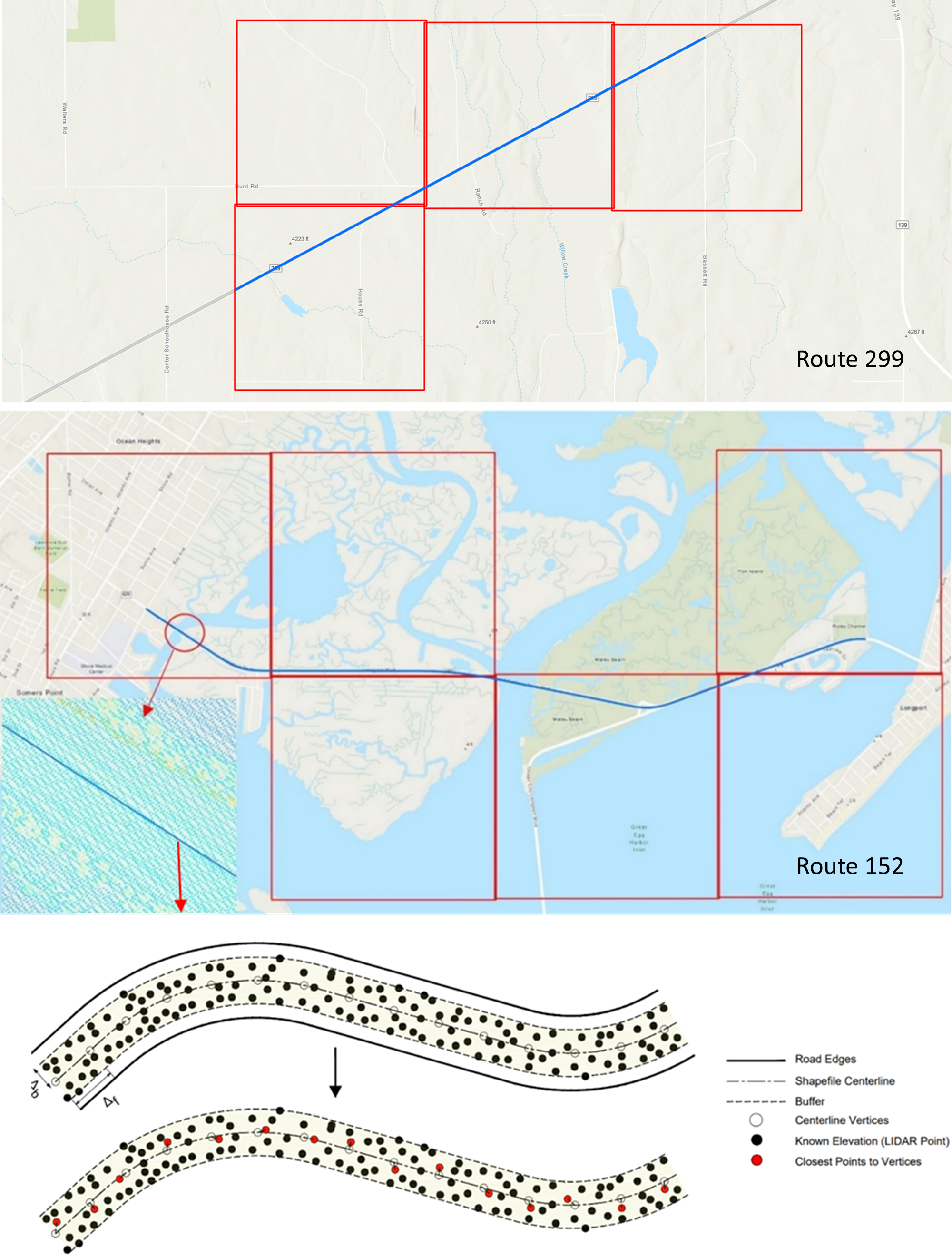
The proposed method was evaluated using the actual vertical alignment data of Route 152, a state highway in Atlantic County, NJ, and Route 299 in Lassen County, CA. The portion of Route 299 starts at (-120.98672, 41.16925) and ends at (-120.96932, 41.17645), and is 1.03 miles in length as depicted in Figure 2a. The portion of Route 152 included for the analysis starts at (-74.58808, 39.31803) and ends at (-74.53119, 39.31595), and is 3.18 miles, as shown in Figure 2b. The vertical alignment consists of 8 curved and 9 tangent segments for Route 299, and 18 curved and 18 tangent segments for Route 152. The selection of these specific portions was due to the availability of the vertical alignment data provided by the New Jersey Department of Transportation (NJDOT) and California Department of Transportation (Caltrans). Figure 2c demonstrates the USGS LiDAR data in the vicinity of the initial segment of Route 152. The elevation can be recognized based on the color scheme, reflecting elevation changes between the road surface and its surroundings.

3.2 Data extraction
This section describes the process of extracting elevation values from LiDAR point cloud data obtained from the USGS data repository. The procedure, illustrated in Figure 3, was conducted using QGIS software. The aerial LiDAR point cloud data were obtained from the USGS as separate files in LAZ format, which is a compressed version of the standard LiDAR point cloud file format. Each LAZ file corresponds to a grid tile of approximately 0.95 by 0.95 miles. The file size was approximately 60 MB for Route 152 and 40 MB for Route 299. The total file size of the files covering Route 152 was approximately 420 Mb, while the corresponding files for Route 299 totaled about 160 Mb. These files contained point cloud data for the entire geographic area encompassed by the tiles.
The procedure used the GIS roadway centerline shapefile of Route 152, publicly available on the NJDOT (NJDOT, 2025) website, and the corresponding roadway centerline shapefile for Route 299, publicly available through Caltrans (Caltrans, 2026), to extract point cloud data exclusively associated with the two study roadways. A buffer width ∆w = 1 meter around the road centerline was used for this purpose. As depicted in Figure 3, the LiDAR points closest to the roadway centerline were then extracted from the buffered point cloud data using QGIS. This process then selected sample points at fixed intervals, ∆f, along the roadway centerline. The choice of ∆f significantly influences the accuracy and efficiency of the elevation extraction process. If ∆f is too long, it may fail to capture essential details of the road elevation profile. Conversely, smaller intervals could lead to increased computational effort. Based on a series of sensitivity analyses, as explained in Section 3.5, it was determined that a 5-meter sampling interval was found to provide an effective balance between accurately representing the vertical alignment and managing the computational effort. A similar sampling strategy was also used by Liu et al. (2018), who selected a 10-meter sampling interval after conducting sensitivity analyses for elevation extraction along roadway centerlines. They noted that excessively short sampling intervals may cause consecutive points to fall within the same DEM grid cell, producing duplicate elevation values, increasing noise in the elevation profile, and adding unnecessary computational effort.
3.3 Overview of the ANN model
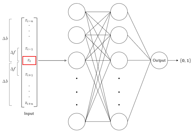
The general overview of the ANN model is presented in Figure 4. The input vector for the ANN model included the elevation (zi) of the target point i, as well as those of its neighbouring vertices. Considering only the elevation of a single LiDAR point, without accounting for its surroundings, is insufficient to accurately determine whether the point belongs to a vertical curve (labelled as 1) or a roadway grade (labelled as 0). Therefore, to improve prediction accuracy, the input vector also incorporated elevation information from the surrounding vertices within a predetermined buffer distance (Δb), as shown in Figure 4.
The limitation of the proposed approach was the need for a substantial amount of real-world alignment data to ensure the ANN model's effectiveness in segmenting different types of roadway alignments. However, as mentioned earlier, obtaining actual road alignment data is challenging. To overcome this limitation, this study utilized synthetically generated random vertical road alignments containing curved and tangent segments. As presented in the next subsection, the synthetic dataset was generated by varying road grades, curve lengths, and curvature transitions to represent realistic combinations of tangents, crest and sag curves. This ensured that the model was trained with diverse geometric conditions and could develop generalized relationships between vertical alignment features and their geometric attributes.
The accurately labelled points of the synthetically generated roads were used to train the ANN model. The following subsection presents the generation of synthetic vertical alignment data.
3.4 Generating synthetic data
The process of generating a synthetic vertical alignment dataset was conducted by a computer code developed in the C programming language. The process can be described briefly as follows. Each generated road started from the origin (0, 0). Each roadway was assumed to contain a specific number of distinct segment types. The type of the first segment, i.e. curve or tangent, was determined randomly. The initial and final grades were randomly assigned between zero and a maximum allowable vertical grade of ±9 percent. The lengths of the initial and final tangent segments were randomly assigned between 150 and 750 feet. Similarly, the curve lengths were randomly assigned between 150 feet and 400 feet. Elevations at any given point along these segments could then be calculated using the fundamental vertical alignment equations (Mannering & Washburn, 2020). An input vector for each point was then generated, as shown in Figure 4, containing the elevation of (zi) of the target point i and its neighbouring points within a given buffer distance (Δb), labelled with the segment type i.e. curved (1) or tangent (0). These vectors were then rescaled by standardization to reduce the size of the search space. Using this process, a total of 40,000 roads were generated, and 20 percent of these points were randomly selected to ensure stochasticity in using the training data for the ANN model.
3.5 Sensitivity Analysis for ANN Model
The training of the ANN model was performed using the synthetically generated vertical alignment dataset described above. The overall dataset included approximately 1,800,000 data points. 80 percent of this dataset was used for training and 20 percent for tuning the model hyperparameters and testing the model.
A series of sensitivity analyses was conducted to evaluate different combinations of ANN model architectures, sampling interval values (Δf), and the distance range used to determine which neighbouring vertices were included in the input vector (Δb). The models were developed using the Keras library within the TensorFlow package in Python. Rectified Linear Unit (ReLU) was used as the activation function, except at the output node where a sigmoid activation function was used. Each model was trained for 50 epochs. Accuracy results of the full sensitivity analysis are summarized in Figure 5.
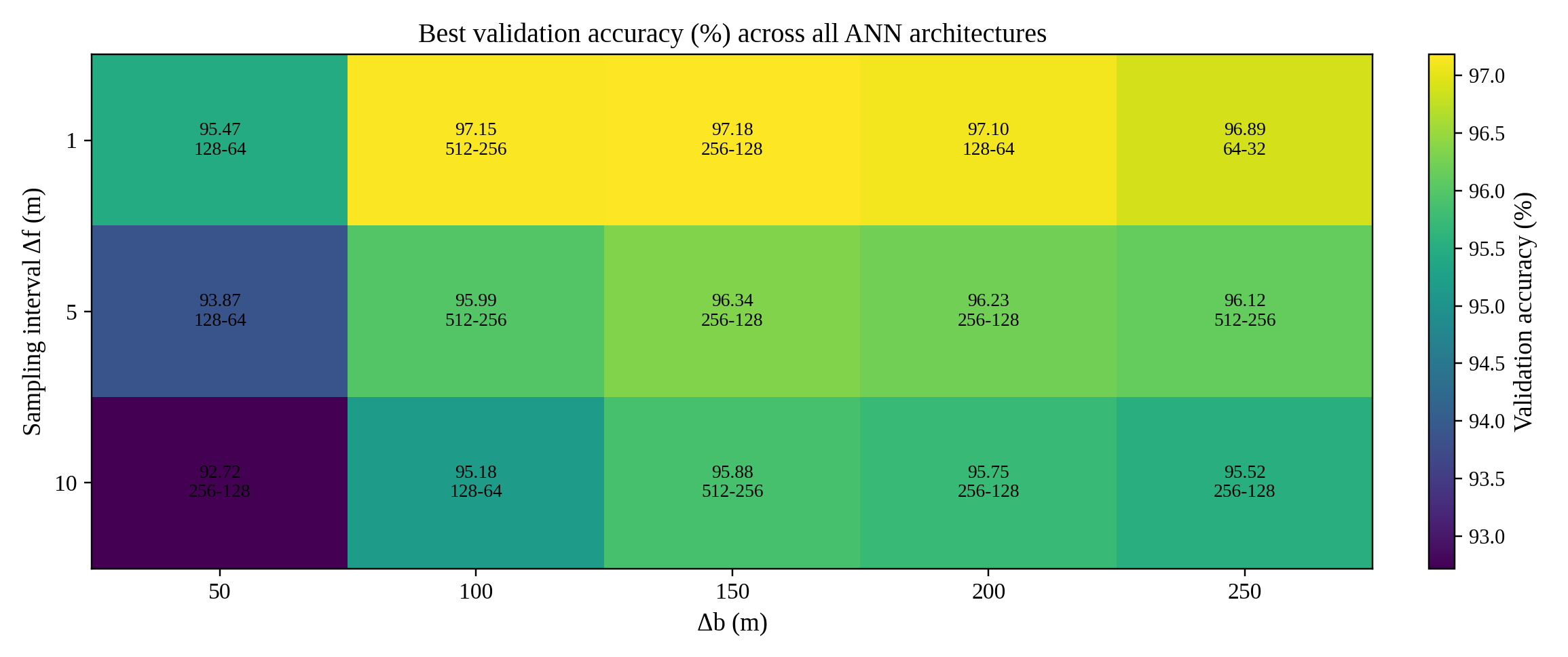
As shown in Figure 5, multiple two hidden-layer ANN structures were tested across combinations of Δf = 1, 5, and 10 m and Δb = 50, 100, 150, 200, and 250 m. Across all tested scenarios, the highest validation accuracy was achieved at Δf = 1 m, reaching 97.18% at Δb = 150 m, while Δf = 5 m yielded a validation accuracy of 96.34% at Δb = 150 m. Thus, the improvement from Δf = 1 m relative to Δf = 5 m was approximately 0.84 percentage points at best. In contrast, reducing the sampling interval from Δf = 5 m to Δf = 1 m increased the number of sampled points and their neighbouring vertices by approximately five times. As a result, the overall data handling and training burden scaled roughly with the product of these effects (approximately 25 times). Given the already large training scale used in this study, the marginal accuracy gain associated with Δf = 1 m did not justify the substantially higher computational cost and reduced scalability. Conversely, Δf = 10 m reduced computational requirements but decreased validation accuracy and increased the risk of under- sampling short vertical transitions. Based on the sensitivity analysis results and the scalability objective of this study, Δf = 5 m and Δb = 150 m (approximately 500 feet) were selected as a practical and effective compromise.
Following the tests with various ANN architectures (Figure 5), the final model was selected as an n-128-64-1 structure, consisting of two hidden layers, and an output layer of one node, where n denotes the size of the input vector. In our analysis, presented in the next section, n = 61 for Δf = 5 m and Δb = 150 m.
4. Analysis results
The selected ANN model was evaluated independently by using the aerial LiDAR data extracted along Route 152 and Route 299 centerlines. The following subsections present the results for the two study roadways separately.
4.1 Analysis of Route 152
The results showed that the ANN model correctly predicted 87.5 percent of the LiDAR points’ labels for Route 152. Further investigation revealed that 82.1 percent of the incorrectly predicted labels were on tangent segments, and the remaining were on curved segments. Also, 88.0 percent of the incorrectly labelled LiDAR points were located in the transition regions between curved and tangent segments. However, the remaining 12 percent corresponded to a total of 14 points, belonging to two clusters, one with six and the other with eight contiguous points. These two clusters were predicted as curved segments. Figure 6 demonstrates these two cases.
In the left plot, all points belonged to a tangent segment based on the actual vertical alignment data, and the red color indicates the points misidentified as belonging to a curved segment (segment number 14 of the estimated data in Table 1).
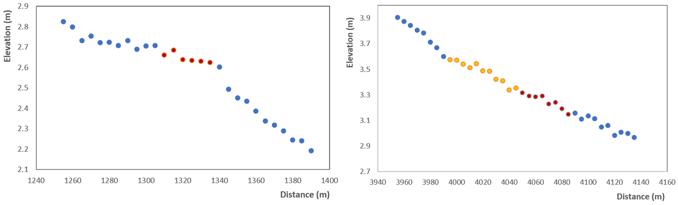
In the right plot, blue and orange points belonged to a tangent and a curved segment, respectively, according to the actual data. However, as seen in the actual data, this 200-feet long curve (segment number 28 of actual data in Table 1) has an initial grade of -0.49 and a final grade of -0.40, which made it indiscernible. The model misidentified a part of the tangent segment after this curve as a separate curved segment. Although a part of this misidentified segment overlaps with the curve before, the remaining portion extends into the following tangent segment. Regardless, it was assumed that the proposed method could not properly detect segment number 28.
Using the predicted labels of LiDAR points, the estimated vertical alignment was generated manually. For example, if the predicted labels indicated a tangent segment, a simple linear regression was conducted using these points, and the grade of a tangent segment was estimated accordingly. It should be noted that although this approach was feasible for a single roadway, an automated process would be more effective if multiple roadways were to be analyzed.
Notably, a key advantage of this approach is its reliance solely on the labelled LiDAR data points, making it easily replicable for other roadway datasets through the application of fundamental vertical alignment equations.
Details of the estimated vertical alignment are presented in Table 1. The total actual tangent and curved lengths were 11,457.5 feet and 5,365 feet, respectively, while the estimated total tangent and curved lengths were 10,477 feet and 6,345.5 feet, respectively. Overall, the proposed method detected all segments except one curve (segment number 28 of actual data in Table 1), and one tangent segment was misidentified as a curved segment (segment number 14 of the estimated data in Table 1).
| Actual | Estimated | ||||||||
|---|---|---|---|---|---|---|---|---|---|
| No | Start | End | Type‡ | Grade (%) | No | Start | End | Type | Grade (%) |
| 1 | 10+00 | 12+40 | T | -0.420 | 1 | 10+00 | 12+35 | T | -0.39 |
| 2 | 12+40 | 14+40 | C | - | 2 | 12+35 | 14+67 | C | - |
| 3 | 14+40 | 18+50 | T | 1.020 | 3 | 14+67 | 18+45 | T | 1.07 |
| 4 | 18+50 | 21+00 | C | - | 4 | 18+45 | 20+40 | C | - |
| 5 | 21+00 | 25+50 | T | -0.530 | 5 | 20+40 | 24+76 | T | -0.59 |
| 6 | 25+50 | 27+50 | C | - | 6 | 24+76 | 28+45 | C | - |
| 7 | 27+50 | 33+50 | T | 0.530 | 7 | 28+45 | 32+55 | T | 0.51 |
| 8 | 33+50 | 35+50 | C | - | 8 | 32+55 | 35+67 | C | - |
| 9 | 35+50 | 42+00 | T | -0.500 | 9 | 35+67 | 41+40 | T | -0.51 |
| 10 | 42+00 | 44+00 | C | - | 10 | 41+40 | 43+70 | C | - |
| 11 | 44+00 | 49+00 | T | 0.500 | 11 | 43+70 | 48+45 | T | 0.42 |
| 12 | 49+00 | 51+00 | C | - | 12 | 48+45 | 50+60 | C | - |
| 13 | 50+60 | 52+90 | T | -0.29 | |||||
| 14† | 52+90 | 53+90 | C | - | |||||
| 13 | 51+00 | 56+00 | T | -0.500 | 15 | 53+90 | 55+35 | T | -0.76 |
| 14 | 56+00 | 58+00 | C | - | 16 | 55+35 | 58+48 | C | - |
| 15 | 58+00 | 65+00 | T | 0.500 | 17 | 58+48 | 64+87 | T | 0.43 |
| 16 | 65+00 | 67+00 | C | - | 18 | 64+87 | 66+85 | C | - |
| 17 | 67+00 | 74+50 | T | -0.500 | 19 | 66+85 | 74+87 | T | -0.47 |
| 18 | 74+50 | 80+50 | C | - | 20 | 74+87 | 80+14 | C | - |
| 19 | 80+50 | 89+00 | T | 4.000 | 21 | 80+14 | 88+84 | T | 4.01 |
| 20 | 89+00 | 102+00 | C | - | 22 | 88+84 | 101+95 | C | - |
| 21 | 102+00 | 110+00 | T | -4.000 | 23 | 101+95 | 110+30 | T | -4.01 |
| 22 | 110+00 | 114+00 | C | - | 24 | 110+30 | 113+87 | C | - |
| 23 | 114+00 | 120+00 | T | -0.500 | 25 | 113+87 | 119+00 | T | -0.52 |
| 24 | 120+00 | 122+00 | C | - | 26 | 119+00 | 122+28 | C | - |
| 25 | 122+00 | 136+50 | T | 0.400 | 27 | 122+28 | 135+35 | T | 0.39 |
| 26 | 136+50 | 138+50 | C | - | 28 | 135+35 | 139+65 | C | - |
| 27 | 138+50 | 141+00 | T | -0.490 | 29 | 139+65 | 142+14 | T | -0.53 |
| 28* | 141+00 | 143+00 | C | - | 30 | 142+14 | 144+10 | C | - |
| 29 | 143+00 | 148+00 | T | -0.400 | 31 | 144+10 | 147+20 | T | -0.40 |
| 30 | 148+00 | 150+00 | C | - | 32 | 147+20 | 150+50 | C | - |
| 31 | 150+00 | 156+00 | T | 0.420 | 33 | 150+50 | 155+40 | T | 0.47 |
| 32 | 156+00 | 158+00 | C | - | 34 | 155+40 | 158+70 | C | - |
| 33 | 158+00 | 169+00 | T | -0.400 | 35 | 158+70 | 169+05 | T | -0.40 |
| 34 | 169+00 | 171+00 | C | - | 36 | 169+05 | 171+00 | C | - |
| 35 | 171+00 | 176+07.5 | T | 0.394 | 37 | 170+00 | 176+25 | T | 0.40 |
| 36 | 176+07.5 | 178+22.5 | C | - | 38 | 176+25 | 178+22.5 | C | - |
However, being able to detect the type of segment should not be used as a decisive evaluation metric as these measures only the existence of, not how much, the overlap between the estimated and actual segments (Bartin et al., 2021; Bartin et al., 2023). Instead, one should measure the ratio of overlap between the estimated curved segments’ lengths and those of the actual ones. Doing so revealed that the overlap ratio of the estimated curve lengths with the actual ones was 92.5 percent, and the same ratio for tangent segments was 87.9 percent. Furthermore, the total undetected lengths of curved and tangent segments were 402.5 feet and 1,383 feet respectively. These corresponded to on average 22.4 feet and 76.8 feet error per curved and tangent segment, respectively. These statistics indicated that the proposed method overpredicted the number of curved points. This can be attributed to the inherent noise in the LiDAR data, as evidenced in Figure 6.
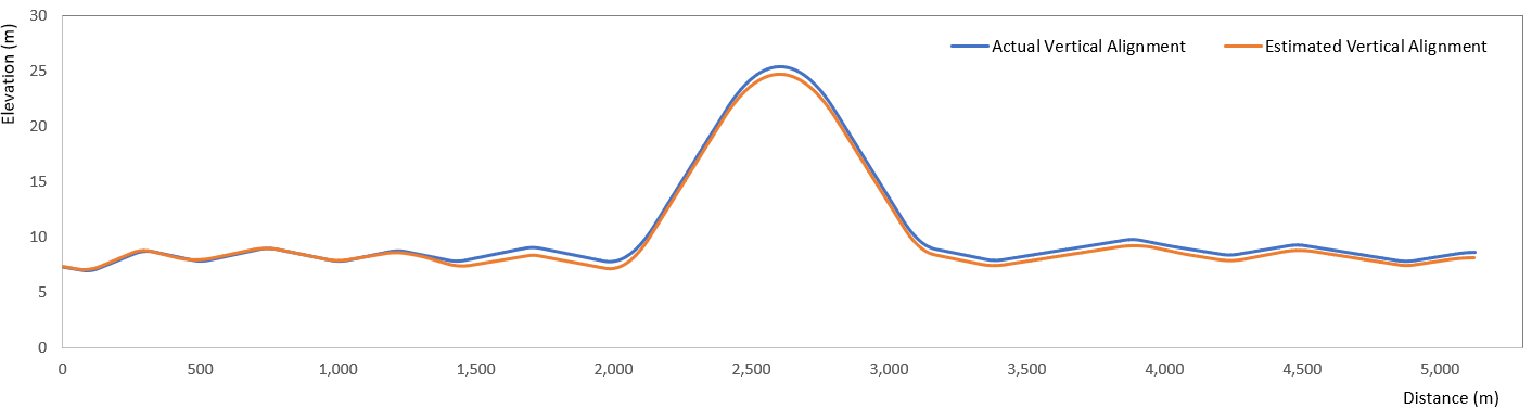
Figure 7 shows the visual comparison of the actual roadway alignment of Route 152 compared to the one estimated by the proposed method. It is worth noting that the start elevation of the LiDAR data was fixed to the actual starting elevation of Route 152 for comparison purposes, since LiDAR only shows the relative elevation and not the actual one.
As shown in Figure 7, the estimated vertical alignment demonstrates an overall acceptable fit with the actual profile; however, an overestimation of the curve length for segment 6 in Table 1 by 169 feet caused the subsequent portion of the estimated alignment to deviate from the actual alignment. Despite this localized accumulation effect, the estimated grades remained accurate, with a mean absolute error of 0.042 percent relative to the actual values, ranging from zero to 0.26 percent.
4.2 Analysis of Route 299
For Route 299, the ANN model correctly predicted 85.93 percent of the LiDAR points’ labels. Among the incorrectly predicted labels, 19.15 percent corresponded to LiDAR points located on tangent segments, while the remainder were on curved segments. Notably, nearly all of the mislabeled LiDAR points occurred within the transition regions between tangent and curved segments. Details of the estimated vertical alignment are presented in Table 2, and the model detected all tangent and curved segments along Route 299; however, slight offsets in the predicted transition points between tangents and curves led to overestimation or underestimation of the lengths of the adjacent tangent and curve segments. The total actual tangent and curved lengths were 2,141 feet and 3,301 feet, respectively, while the estimated total tangent and curved lengths were 2,522 feet and 2,920 feet, respectively. The overlap between the actual and estimated segment types along the roadway was 87.2 percent. The overlap ratio of the estimated curve lengths with the actual ones was 83.7 percent, and the corresponding ratio for tangent segments was 92.7 percent. Furthermore, the total undetected lengths of curved and tangent segments were 538 feet and 157 feet, respectively, which corresponded to an average error of 67.3 feet per curved segment and 17.4 feet per tangent segment. Overall, these findings suggest that the proposed method tended to underestimate the extent of curved segments, which may be attributed to the relatively small grade differences across several vertical curves in Route 299, causing portions of curves to be misidentified as tangent, particularly near transition regions.
| Actual | Estimated | ||||||||
|---|---|---|---|---|---|---|---|---|---|
| No | Start | End | Type‡ | Grade (%) | No | Start | End | Type | Grade (%) |
| 1 | 1237+58 | 1239+83 | T | 0.71 | 1 | 1237+58 | 1240+52 | T | 0.77 |
| 2 | 1239+83 | 1244+33 | C | - | 2 | 1240+52 | 1244+14 | C | - |
| 3 | 1244+33 | 1247+15 | T | -0.48 | 3 | 1244+14 | 1247+58 | T | -0.64 |
| 4 | 1247+15 | 1250+55 | C | - | 4 | 1247+58 | 1250+86 | C | - |
| 5 | 1250+55 | 1252+33 | T | -2.12 | 5 | 1250+86 | 1252+83 | T | -2.32 |
| 6 | 1252+33 | 1255+54 | C | - | 6 | 1252+83 | 1255+62 | C | - |
| 7 | 1255+54 | 1257+81 | T | -0.13 | 7 | 1255+62 | 1258+24 | T | -0.075 |
| 8 | 1257+81 | 1259+81 | C | - | 8 | 1258+24 | 1259+88 | C | - |
| 9 | 1259+81 | 1260+82 | T | -3.48 | 9 | 1259+88 | 1261+03 | T | -3.81 |
| 10 | 1260+82 | 1263+52 | C | - | 10 | 1261+03 | 1264+15 | C | - |
| 11 | 1263+52 | 1264+40 | T | 0.28 | 11 | 1264+15 | 1265+30 | T | 0.22 |
| 12 | 1264+40 | 1272+10 | C | - | 12 | 1265+30 | 1271+37 | C | - |
| 13 | 1272+10 | 1276+25 | T | -0.20 | 13 | 1271+37 | 1276+78 | T | -0.16 |
| 14 | 1276+25 | 1279+25 | C | - | 14 | 1276+78 | 1279+73 | C | - |
| 15 | 1279+25 | 1281+39 | T | 4.24 | 15 | 1279+73 | 1281+87 | T | 4.43 |
| 16 | 1281+39 | 1287+89 | C | - | 16 | 1281+87 | 1287+60 | C | - |
| 17 | 1287+89 | 1292+00 | T | -1.42 | 17 | 1287+60 | 1292+00 | T | -1.21 |
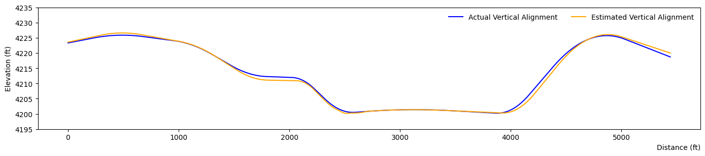
As shown in Figure 8, the estimated alignment follows the actual profile with an overall acceptable fit; however, the overestimation of the tangent grades between segments 6 and 10 caused a noticeable deviation from the actual alignment. In addition, another deviation occurred after segment 12, where the estimated curve length was shorter than the actual by 163 feet. This shortening causes the subsequent portion of the estimated profile to progressively drift relative to the actual alignment. Despite these localized discrepancies, grade estimation performance remained strong, with the absolute error between actual and estimated grades varying between 0.04 to 0.33 percent across the evaluated segments with a mean absolute error of 0.15 percent.
4.3 Summary of Analysis Results
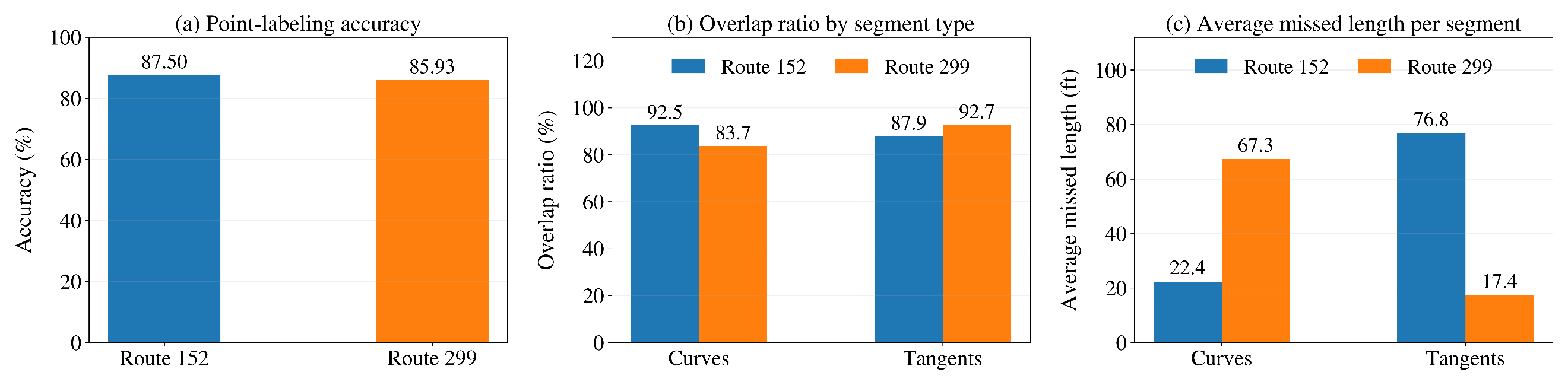
Figure 9 summarizes the key performance metrics for the two evaluated roadways. The ANN achieved labelling accuracy of 87.5 percent for Route 152 and 85.93 percent for Route 299. Route 152 showed higher overlap for curves than for tangents, with overlap ratios of 92.5 percent and 87.9 percent, respectively; in contrast, Route 299 showed higher overlap for tangents than for curves, with overlap ratios of 92.7 percent for tangents and 83.7 percent for curves. This pattern is consistent with the average missed lengths. Route 152 had a larger average missed tangent length, 76.8 ft, but a smaller missed curve length, 22.4 ft, while Route 299 showed the opposite behavior, with 67.3 ft missed per curve segment and 17.4 ft per tangent segment.
4.4 Comparative Studies
The proposed ANN-based vertical alignment estimation method was compared with the DEM-based grade estimation method introduced by Liu et al. (2018). They proposed a method to obtain roadway grade from the DEM, using elevation extraction along road centerlines, cleaning and infilling erroneous elevation artifacts, applying cubic smoothing splines to reduce noise, and calculating grade as the derivative of the resulting elevation profile. Liu et al. (2018)’s approach generates a continuous grade profile and does not directly provide tangent/vertical-curve labelling or vertical-curve geometric parameters. The study used mean absolute error (MAE) as the performance metric when evaluating the accuracy of the grades on tangent segments.
Accordingly, the comparison in this study focused on the accuracy of tangent grade estimation on the two independent roadways, namely Route 152 and Route 299. The results are summarized in Table 3. For Route 152, the proposed method achieved an MAE of 0.042 percent, compared with 0.057 percent obtained using the DEM-spline method. For Route 299, the proposed method achieved an MAE of 0.145 percent, compared with 0.188 percent for the DEM-spline method. In addition to improved grade estimation accuracy, the proposed method also provides pointwise tangent and vertical curve labels that support vertical alignment segmentation and curve identification, enabling the extraction of segment-level vertical alignment characteristics reported in Table 1 and Table 2.
| Roadway | Proposed Method MAE (%) | Liu et al. (2018) Method MAE (%) | Proposed Method Max error (%) | Liu et al. (2018) Method Max error (%) |
|---|---|---|---|---|
| Route 152 | 0.042 | 0.057 | 0.26 | 0.25 |
| Route 299 | 0.145 | 0.188 | 0.33 | 0.64 |
4.5 Case study
To demonstrate the practical application of LiDAR derived vertical alignment data, case studies were conducted on two rural two-lane roadways: Route 299, presented in the previous section, and Route 83 in Cape May County, NJ, which was examined as an independent case study. The primary objective was to use the extracted vertical alignment data to conduct a speed safety assessment along the roadway and identify locations where speed reductions may be warranted due to limited sight distance or sharp curvature. Because posted speed limits are often established at the time of roadway construction and may not be periodically reassessed, the proposed approach can also be used to reevaluate the appropriateness of speed limits for individual roadway segments based on current geometric conditions estimated using LiDAR data.
To determine the advisory speed governed by roadway geometry, we first divide the alignment into discrete segments based on changes in vertical grade (tangents vs. vertical curves) and horizontal curvature (tangents vs. horizontal curves).
For each vertical-curve segment i of length Li and average absolute grade Gi, we compute the maximum safe stopping speed Vv,i by equating the stopping-sight distance to the curve length under a conservative braking deceleration d, following standard highway design procedures (AASHTO, 2011):
\begin{equation} V_{v,i} = \sqrt{2gL_{i}}(d+G_i),\quad d = 0.347g\tag{1} \end{equation}This formula captures the combined effect of gravity and grade on required stopping distance along the curve. For horizontal curves of radius Ri, we apply the standard rural-road speed formula with superelevation e = 0.06 and side-friction f = 0.15 (AASHTO, 2011).
\begin{equation} V_{h,i} = \sqrt{127R_{i}}(e+f)\tag{2} \end{equation}Each roadway segment was analyzed independently, and the minimum of the vertical and horizontal speeds, subject to the statutory speed limit, was assigned as the regenerated speed.
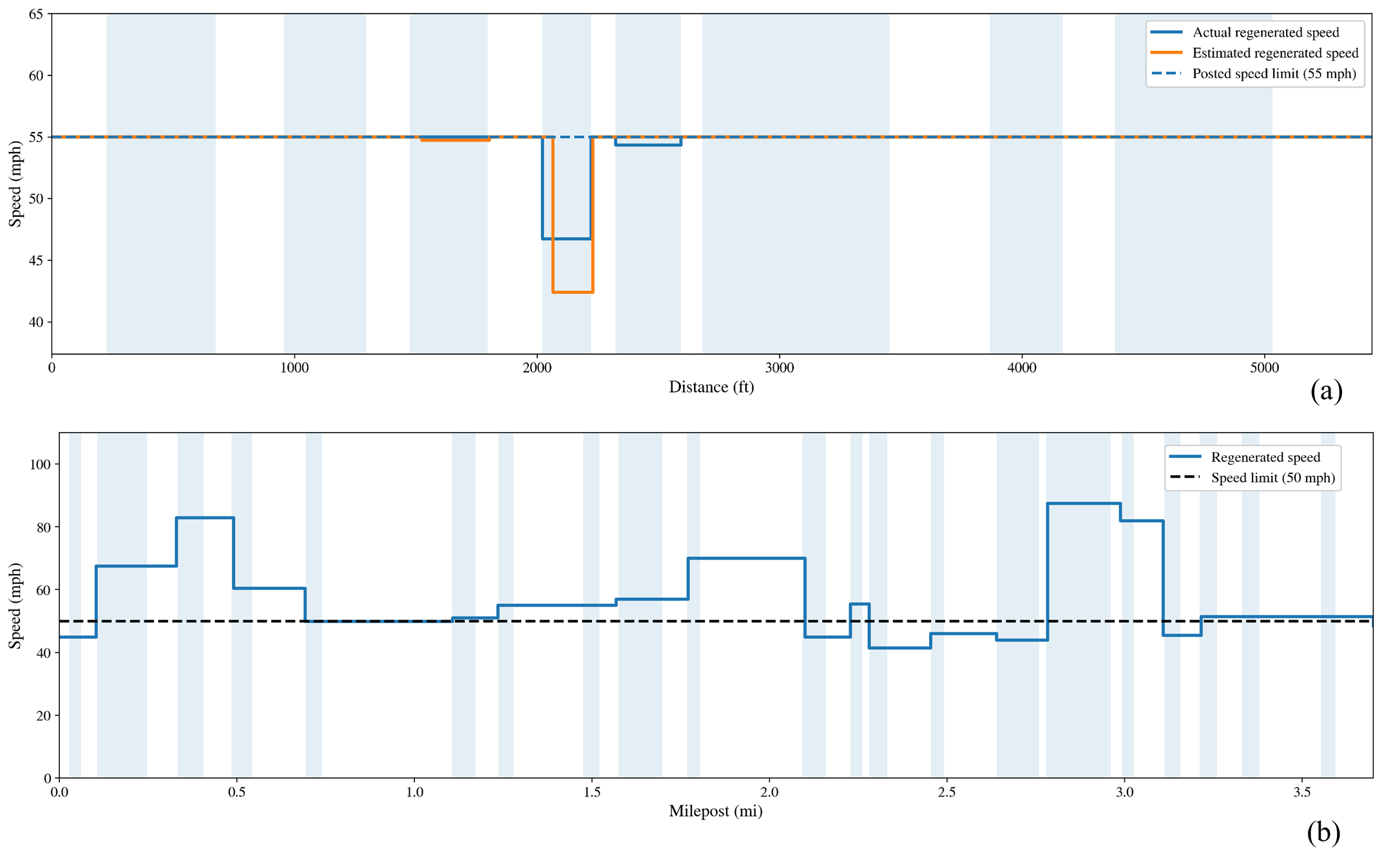
Route 299 was evaluated using both the actual vertical alignment and the ANN-estimated vertical alignment. The portion of Route 299 analyzed in this study is located on a straight section where there are no horizontal curves; therefore, the regenerated speed profile was governed by the vertical alignment only (Equation 1). The posted speed limit along the selected portion of Route 299 is 55 mph. Figure 10a illustrates the regenerated speed profile computed along Route 299 using the actual and estimated vertical alignment data. The dashed black line indicates the speed limit (55 mph), while the stepwise regenerated speed profiles show the segment-based speeds computed from the vertical alignment. Shaded regions correspond to actual vertical curve regions. As seen in Figure 10a, most segments remain at the posted speed limit, indicating that the vertical geometry along this portion of the corridor generally does not impose substantial stopping-sight constraints. However, a localized reduction occurs at a short vertical-curve segment (Segment 8), which controls the minimum regenerated speed in the corridor. Using the actual vertical alignment, this segment yielded a regenerated speed of approximately 46.7 mph, while the estimated vertical alignment yielded a lower regenerated speed of approximately 42.4 mph. This difference is attributable to the estimated vertical alignment representing the controlling curve as slightly more restrictive, which reduces the stopping-based speed computed from Equation 1. Overall, the results for Route 299 indicate that the proposed method can correctly identify the roadway location that governs the minimum safe speed while also providing a conservative estimate of that speed when the roadway alignment is derived from estimated data.
Route 83 is a 3.79-mile-long rural highway. Its horizontal alignment data were extracted from as-built plan files provided by the NJDOT, and documented in detail by Bartin et al. (2022), which consists of 22 segments: 11 horizontal curves and 11 tangents. Curve segments account for approximately 5,298 ft (~1.00 mi), averaging about 482 ft each, with radii ranging from 385 ft to 6,910 ft, with an average of 2,881 ft. However, the vertical alignment of Route 83 was not available in the as-built plan files. Thus, following the same analysis steps presented in Section 3, its vertical alignment was estimated using the corresponding USGS LiDAR data. The estimated vertical alignment for Route 83 consisted of 42 vertical segments, of which 21 were vertical curves. Together these curves totaled about 1.31 miles, with an average length of nearly 328 ft per curve. Tangent sections exhibited modest slopes, averaging just over 1.07 %, while the vertical-curve segments had an average rate of grade change of approximately 1.06 %.
Figure 10b illustrates the speed profile regenerated along Route 83. The regenerated speed limits were mostly constrained by the vertical alignment rather than the horizontal, primarily because the horizontal curves along Route 83 do not impose significant speed limitations. In contrast, the estimated vertical curves were relatively short and steep, which restricted stopping sight distance and necessitated speed reductions. Therefore, Figure 10b highlights only the vertical curve regions where speed reductions occurred due to vertical alignment constraints. The dashed black line shows the speed limit (50 mph), while the blue line represents the regenerated speed limits computed for each vertical curve segment. As seen, several segments along the roadway required speed reductions, especially where steep or abrupt crest vertical curves were present. These segments represented critical points where limited sight distance could compromise safety, and therefore might benefit from countermeasures such as advisory signage or speed control strategies.
It should be noted that the higher speeds shown in certain segments in Figure 10 were based on geometric analysis only, using vertical and horizontal alignment characteristics. In practice, additional factors such as intersections, pavement condition, lane width, roadside environment, and driver behaviour may also influence operating speeds and posted limits. Despite these limitations, this case study demonstrates how publicly available USGS LiDAR and ANN based vertical alignment estimates can support network-level safety assessments by identifying segments where geometric conditions impose speed constraints. The same methodology can be applied across other roadways using the widely available USGS LiDAR data and the proposed framework.
5. Conclusions
Roadway vertical alignment data play a crucial role in a wide range of highway engineering and safety applications. Vertical grades and curvature shape sight distance, operating speeds, driver workload, and vehicle dynamics, and thus underpin both geometric design decisions and crash modelling. Guidance from AASHTO and FHWA highlights the decisive role of grade and crest–sag curvature in determining stopping sight distance, maintaining speed consistency, and managing visibility limitations on vertical curves (Donnell et al., 2018). Empirical evidence further shows that steep grades, combined with horizontal and vertical curvature, increase crash risk and disrupt speed uniformity, especially on rural two-lane roads (Elvik & Haugvik, 2023; Ryan et al., 2022; Bauer & Harwood, 2013; Papadimitriou et al., 2019; Kar et al., 2024). Beyond safety, vertical alignment influences drainage design, fuel consumption, ride comfort, and maintenance strategies, and supports three-dimensional roadway coordination and visibility assessments (FHWA, 2019).
Despite its importance, obtaining vertical alignment data at scale remains difficult and expensive. Legacy plans and profile sheets are often non-digital, and precision surveys using GPS, GNSS, or mobile LiDAR require specialized equipment and substantial resources, limiting corridor coverage (Gargoum & El Basyouny, 2019). While horizontal alignment can be traced using open geospatial layers or imagery, vertical profiles cannot be inferred without elevation data, which complicates coverage across large networks.
Recent advances in remote sensing help mitigate these barriers. The USGS 3DEP program provides nationwide point clouds and DEMs via The National Map, enabling low-cost derivation of elevations and slopes for most U.S. roads (USGS, 2025). Prior work demonstrates the promise of LiDAR for automated geometry extraction and safety assessment (Yang & Das, 2024; Gargoum & El Basyouny, 2019; Wang et al., 2025), but network-scale processing, roadway point isolation, and reliable classification of tangents and vertical curves still require robust, scalable analytics.
In this context, this study introduced an innovative approach to estimating vertical alignment data of roadways, which combines LiDAR data with an ANN model, addressing a critical gap by providing an efficient, scalable, and reproducible way to estimate roadway vertical alignment characteristics. Extraction of vertical alignment is known to be time-consuming and expensive, thus necessitating an efficient and rapid method due to its vital role in various traffic safety-related analyses.
Prior research on the acquisition of road elevation data has predominantly centered on the utilization of GPS and GNSS data from vehicles equipped with sophisticated technologies. Nevertheless, the requirement of such specialized surveying vehicles for data gathering has constrained the method's relevance to a broader array of road networks, owing to substantial costs and prolonged data collection periods. The proposed approach capitalizes on the aerial LiDAR data on the USGS website (USGS, 2025), which covers the majority of roads in the US.
An ANN-based approach was used to detect and identify distinct segment types along a road’s vertical alignment. First, LiDAR data were processed and the points corresponding to the study road were extracted using QGIS. Although applied to one roadway, a similar process can be repeated for multiple roads efficiently in a short period of time. Each LiDAR point's classification, indicating whether it corresponded to a vertical tangent or curved segment, was predicted through the proposed ANN model. These predicted classifications were then utilized to estimate the number and characteristics (tangent or curved) of the road segments.
To train the ANN model, synthetically generated vertical road alignment data were employed. The results of the segmentation process were used to determine essential geometric parameters such as segment length and grades. The key advantage of the presented approach is that it relies only on the labelled LiDAR data points, which makes it easily replicable for other roadway datasets.
The test dataset employed in this study comprised the vertical alignment data of Route 152 in NJ and Route 299 in CA, both two-way two-lane rural roadways. The results of the analyses demonstrated a strong agreement with the actual alignment (See Figure 7 and Figure 8). As shown in the summary of evaluation results presented in Figure 9, for Route 152, an overlap of 92.5 percent with the curved segments’ lengths and 87.9 percent with the tangent segments’ lengths was achieved, indicating a high level of concurrence between the estimated and actual segments. For Route 299, the overlap of the estimated alignment with the actual one was 83.7 percent for curved segments and 92.7 percent for tangent segments. Regarding the evaluation metrics, the average undetected segment lengths were determined to be 22.4 feet and 76.8 feet for curved and tangent segments, respectively for Route 152, while the corresponding values were 67.3 feet and 17.4 feet for curved and tangent segments, respectively, for Route 299.
Furthermore, the mean absolute error between the estimated and actual grades was found to be 0.042 percent, with variations ranging from 0 percent to 0.26 percent, for Route 152. For Route 299 the mean absolute error was 0.15 percent, with variations ranging from 0.04 percent to 0.33 percent, thus indicating a generally accurate estimation of grades in the analysis.
As mentioned earlier, roadway vertical alignment datasets are essential in various safety analyses. To demonstrate this, a case study was conducted for Route 83 in NJ and Route 299 in CA, where the extracted vertical alignment data were used to regenerate speed profiles and to identify segments requiring speed reductions. The satisfactory estimation results of this study indicate that the proposed approach can be employed for conducting large-scale analyses to estimate vertical alignment data.
Future work will involve comparing aerial and drone-based LiDAR to evaluate differences in resolution, accuracy, and cost for various roadway types. A comparison between DEM and raw point cloud data can also help determine which source better captures subtle vertical transitions. Additionally, developing an automated framework to estimate vertical alignment across multiple roadways would enable efficient, large-scale analysis and support broader safety assessments.
Acknowledgements
The contents of this paper only reflect the views of the authors, who are responsible for the facts and do not represent any official views of any sponsoring organizations or agencies.
Competing interests
The authors report no competing interests.
CRediT contribution
Mojibulrahman Jami: Conceptualization, Data curation, Formal analysis, Investigation, Methodology, Writing—original draft, Writing—review & editing. Bekir Bartin: Conceptualization, Data curation, Formal analysis, Investigation, Methodology, Writing—original draft, Writing—review & editing. Kaan Ozbay: Conceptualization, Formal analysis, Investigation, Methodology, Writing—original draft, Writing—review & editing.
Ethics
This study did not involve human participants, or identifiable personal data and relied solely on publicly available geospatial datasets (e.g., USGS 3DEP LiDAR).
Funding
The study is supported by the NJDOT (FHWA-NJ-2017-007) and partially by Ozyegin University and partially by C2SMARTER, a Tier 1 UTC at New York University funded by the USDOT.
Generative AI use in writing
During the preparation of this work, the authors used ChatGPT (OpenAI) in order to improve the clarity, grammar, and wording of specific sections of the manuscript. The output was reviewed and revised by the authors, who take full responsibility for the content of the publication.
Editorial information
Handling editor: Lai Zheng, Harbin Institute of Technology, China.
Reviewers: Peijie Wu, Chongqing Jiaotong University, China; Feng Jiang, Harbin Institute of Technology, China.
Submitted: 20 October 2025; Accepted: 22 March 2026; Published: 3 April 2026.