The logic of empirical testing of accident prediction models
Abstract
This paper explains the logic of empirical testing of accident prediction models. The key element of empirical testing is to make out-of-sample predictions of the number of accidents. This means that a model developed in sample A is applied, without modification, to predict the number of accidents in sample B. The procedure is illustrated in two samples formed by randomisation. A model fitted to the first sample was applied to predict the number of accidents in the second sample. The model was only partly supported. In general, any accident prediction model is likely to be merely a local statistical description of a particular data set. If tested by means of out-of-sample predictions, the model is very likely to be falsified. This does not mean that accident prediction models do not show general tendencies, but these tendencies are likely to be empirically supported only at a qualitative level, or at best an ordinal level of numerical measurement. In this sense accident prediction models are similar to many models developed in economics. The models predict the direction, and in some cases the relative strength of statistical relationships, but not their precise numerical values.
1. Introduction
Accident prediction models, developed by means of negative binomial regression or related techniques, have become an important tool for road safety analysis and planning. Hundreds of accident prediction models have been developed, and have been applied, for example, to predict the number of accidents for junctions or road sections with known traffic volume and other characteristics. The Highway Safety Manual relies on accident prediction models to estimate the expected number of accidents for various types of highways and intersections. However, there is surprisingly little information about how accurate the predictions made by accident prediction models are. Do such models predict well in data sets that were not used to develop the models? If not, how wrong must predictions be to conclude that a model is wrong, or falsified? How can criteria for confirmation and falsification of accident prediction models be defined and evaluated? In other words: what is the logic of empirical testing of accident prediction models?
A search for studies discussing this problem did not produce a single positive finding. Remarkable as it is, not a single of the hundreds of accident prediction models appears to have been tested empirically. The problem is never even mentioned. Perhaps a reason for this, is that studies that might be interpreted as empirical tests of accident prediction models use the words “calibration” or “transferability” to refer to the analyses performed (see e.g. Sawalha and Sayed 2006, Srinivasan et al. 2013, 2016, Farid et al. 2016, Tang et al. 2020, Avelar et al. 2021, La Torre et al. 2022). Calibration, introduced in the Highway Safety Manual (AASHTO 2010), denotes adjusting the predictions of a model by multiplying them with the ratio between the observed and predicted number of accidents. Initially, a single calibration factor was applied to all units of observation for which an accident prediction was sought. Subsequently, more advanced calibration methods were developed (Srinivasan et al. 2016), enabling unique calibrated values to be estimated for each unit of observation. Analyses of transferability focus on estimated model parameters (coefficients). There are two main types of parameters: the scale parameter (constant term) and the shape parameters (parameters for each of the variables included in a model). Calibration typically starts by adjusting the scale parameter. If this results in a good fit to the data, the other parameters are left unchanged. If the model still does not fit well, one or more of the shape parameters may also be adjusted. The objective of the analysis is to find a model that fits the data well. As will become clear later in the paper, such an analysis does not represent an empirical testing of a model, since the objective is only to find a set of parameter values that describe a given data set better than any other set of parameter values. Analysts are, as it were, proposing hypotheses after looking at the data and aim to formulate those hypotheses that are most consistent with the data. Empirical testing, on the other hand, makes predictions that may turn out to be wrong, i.e. imply the falsification of a model. Empirical testing requires criteria of falsification, that is statements defining those observations that will lead the analyst to conclude that a model has been falsified.
Following a brief review of some studies evaluating the transferability of accident prediction models, the logic of empirical testing of such models is explained more in detail and falsification criteria are proposed. The main objective of the paper is to explain the logic of empirical testing of accident prediction models and illustrate how such a test can be performed.
2. Review of studies of transferability of accident prediction models
Studies evaluating the transferability of accident prediction models come closer to empirical testing of the models than calibration studies. However, these studies do not formulate explicit criteria of falsification, which would amount to criteria specifying a failure to identify any method for transferring an accident prediction model with sufficiently accurate results. The notion of “sufficiently accurate results” is not very precise and has been interpreted differently in different studies.
Sawalha and Sayed (2006) studied whether an accident prediction model developed for the city of Vancouver could be transferred to the city of Richmond. Three methods for transferring were compared. It was concluded that a maximum likelihood method, which adjusted the shape parameter of the negative binomial distribution (this parameter is the inverse of the over-dispersion parameter) and the constant term of the accident prediction model gave the most accurate results. Accuracy was assessed only by means of a summary statistic and no data were presented on the accuracy of the transferred model for each street section.
Farid et al. (2016) proposed to use the empirical Bayes method to adjust the results of a transferred accident prediction model. They noted, however, that there is an element of self-contradiction in this procedure, since it assumes that data on the recorded number of accidents, which could serve as the basis for developing a local accident prediction model, are available. However, it is difficult to understand how the precision of a transferred accident prediction model can be assessed at all if no accident data are available. At any rate, Farid et al. found that adjusting model predictions by means of the empirical Bayes method gave more precise predictions. This is hardly surprising, as no model contains all variables that are related to the number of accidents. Thus, the recorded number of accidents contains some information on the site-specific effects of variables not included in the accident prediction model.
Tang et al. (2020) introduced a learning algorithm to improve the transferability of accident prediction models. The use of this algorithm did improve the accuracy of a transferred model, but the reported mean square prediction errors remained quite large. Diagrams presented in the paper indicate large prediction errors. Indeed, errors of the magnitude shown in Figure 3 of the paper by Tang et al. would normally justify concluding that the transferred model has been falsified, since it in most cases does not predict correctly and in many cases very erroneously.
La Torre et al. (2022) evaluated the transferability of the Highway Safety Manual (HSM) accident prediction model for freeways to a sample of European countries. Their main conclusion was that developing jurisdiction-specific accident prediction models, i.e. models for each country, produced more precise predictions than those obtained by transferring the HSM model. This result goes a long way towards rejecting the entire notion of transferability and suggesting that unique accident prediction models should be developed for each data set for which a need is felt for such models.
3. The logic of empirical testing of theories
It is an aim of most branches of science to uncover lawlike relationships. Some branches of science deny the existence of lawlike relationships. Historians, in particular, argue that searching for universal causes of revolutions or war makes no sense, as each revolution or war has its particular causes. Nevertheless, statistical regularities can be observed in many historical data sets. These regularities may be somewhat noisy and should not be viewed as anything nearly as well-established as the laws of natural science. Still, the existence of the regularities ought to challenge researchers into developing the most parsimonious general description of them.
Accident research is placed somewhere between the pure natural sciences and history as far as the existence of lawlike relationships is concerned. It ought to be possible to develop accident prediction models containing rather few terms referring to variables for which data are normally available and subject the models to empirical testing. In a classic paper in economics, Milton Friedman (1953) discussed the logic of testing scientific hypotheses. He stated the following regarding the logic of such tests:
“The only relevant test of the validity of a hypothesis is comparison of its predictions with experience. The hypothesis is rejected if its predictions are contradicted; it is accepted if its predictions are not contradicted.”
He continued:
“Truly important and significant hypotheses will be found to have “assumptions” that are wildly inaccurate descriptive representations of reality, and, in general, the more significant the theory, the more unrealistic the assumptions (in this sense). … The relevant question to ask about the “assumptions” of a theory is not whether they are descriptively “realistic”, for they never are, but whether they are sufficiently good approximations for the purpose in hand. And this question can be answered only by seeing whether the theory works, which means whether it yields sufficiently accurate predictions.”
In economics, it is often assumed that consumers or producers are perfectly rational. Friedman accepted that this assumption is often descriptively inaccurate but maintained that hypotheses based on it can be accepted if their empirical predictions are supported by data.
When developing accident prediction models, researchers take great care to develop models that fit the data as closely as possible. Tools to help ensure this (the integrate-differentiate tool and the cumulative residuals plot tool) have been developed by Hauer and Bamfo (1997). Other approaches intended to help develop models that fit the data well include the choice of probability distribution for accidents (Poisson, negative binomial, Posson-lognormal, negative binomial-Lindley, etc.), variable transformations (natural logarithm, square terms, square root terms, etc.), use of interaction terms (variables multiplied by each other), use of random parameter models (Mannering, Shankar and Bhat 2016), or modelling the accident generation process as having more than one modality (e.g. a zero or low-mean state in addition to the normal state) (Lord and Mannering 2010). The widespread use of these tools shows that in accident modelling, getting the assumptions right, i.e. developing a model which is as descriptively accurate as possible is an important analytic objective. This approach to model development is in major contrast to the use of highly simplifying assumptions in economic models.
The great emphasis put on descriptive accuracy in accident prediction models can perhaps be traced to the fact that: “There is no theory behind Equation 1 (an accident prediction model for intersections, my remark), there are no good reasons for which it has been chosen, and there are many functions that would fit the data just as well or better but yield different extrapolated values” (Hauer 2025:10). If models cannot be based on theory, they must be based on data and made to fit the data as well as possible. It is only by developing and comparing models for different data sets that one may learn whether a particular type of model, or family of models, has any general validity.
These points of view are too pessimistic. It is of course correct that there are no theories of accident causation that are as general and concise as the theory of rationality in economics or the theory of gravity in physics. It is, however, not true that no conceptual framework can be developed that impose reasonable constraints on both: (1) the variables to be included in an accident prediction model and (2) the functional form of the relationship between these variables and the number of accidents.
This paper applies an accident prediction model for junctions to explain the logic of empirical testing of such models. The next section therefore discusses whether there is any theoretical basis for defining a basic general form for an accident prediction model for junctions.
4. Theoretical guidance for accident prediction models
Elvik, Erke and Christensen (2009) and Elvik (2010, 2015) discuss elementary units of exposure and their relationship to accident occurrence. An elementary unit of exposure is any countable event that has the potential of generating a traffic conflict. One such event is the simultaneous arrivals at a junction from conflicting directions of two or more vehicles or road users. One of the vehicles or road users must then give way to the other to avoid a conflict or accident. If a simultaneous arrival is defined as arrival within the same second, it can be shown that the number of simultaneous arrivals that have the potential of generating a conflict increases much faster than the number of vehicles entering a junction. Thus, if the number of entering vehicles increases by a factor of 20 in a three-leg junction, the number of simultaneous arrivals increases by a factor of 228.5. However, most of these simultaneous arrivals will not result in a conflict, because road users can predict (most of) the arrivals and adapt their behaviour to them. Elvik (2010, 2015) refers to this kind of behavioural adaptation as learning: the repeated exposure to a certain event teaches road users how to behave in that event to avoid a conflict or accident.
Learning is never perfect. Therefore, some of the simultaneous arrivals develop into conflicts in which fast action must be taken to avoid an accident. A few of the conflicts are detected too late to avoid an accident. There is, however, sufficient statistical regularity in the occurrence of events and road user adaptation to them to propose a number of hypotheses about the sign and magnitude of coefficients in accident prediction models for junctions. It is assumed that the number of entering vehicles is known for all approaches. It is further assumed that the number of legs in the junction is known, the type of traffic control is known, and the speed limit is known. It is assumed that the number of entering vehicles is stated in terms of its natural logarithm (ln). Transforming continuous variables to their natural logarithms is very common in accident modelling. The following hypotheses are proposed:
H1: The sum of the coefficients for major and minor entering volume will have a value greater than 1. Both coefficients will be positive.
H2: The values of the coefficients for entering volume will be nearly proportional to the shares represented by major road and minor road entering volume, although with a slightly higher than proportional value for minor road entering volume.
H3: The coefficient for the number of legs will be positive.
H4: The coefficients for speed limit (assumed to be represented by a set of dummy variables) will indicate a consistent increase in the number of accidents as speed limit increases.
All hypotheses are subject to the “all else equal” clause. If, for example, the sum of the coefficients for entering volume is 1.1, one might expect a coefficient close to 0.8 for major road entering volume and close to 0.3 for minor road entering volume in junctions where, on average, 80 % of vehicles enter from the major approaches and 20 % enter from the minor approaches. It is reasonable to expect that there will be a “safety-in-numbers” effect for minor road entering volume, meaning that if it increases from, say, 20 % to 40 %, the value of the coefficient for minor road volume will not double, but might increase from 0.3 to 0.45. The coefficient for major road entering volume might decrease, for example from 0.8 to 0.7.
Accident prediction models where the coefficients satisfy the constraints implied by the above hypotheses will be judged as theoretically plausible. Again, however, using such a formulation does not suggest that some highly developed theory supporting precise predictions of coefficient values exists. The hypotheses are only a framework for assessing whether a set of coefficients have plausible values. They are what Elvik and Høye (2023A) referred to as “low-level” theory.
5. The random split half method
A data set including 730 rural junctions in Norway, with data for 1997-2002 (Kvisberg 2003) is used to illustrate the logic of empirical testing of accident prediction models. For each junction, data on the following variables was available:
-
Major road entering volume
-
Minor road entering volume
-
Number of legs (3 or 4)
-
Speed limit (40,50,60,70,80,90 km/h)
-
The number of injury accidents during 1997-2002
All junctions were controlled by yield signs on the minor approaches. To create a data set for testing how well an accident prediction model predicts accidents in a data set not used to develop the model, the junctions were randomly split into two equally large groups. This was done by running the “random between 0 and 1” routine in Microsoft Excel. This routine generates either 0 or 1 at random. Since no two random samples of the numbers 0 and 1 will be identical, the routine was run nine times. This generated a 730 rows by 9 columns matrix of 0 and 1. For each row, a sum was computed. If it was 5 or greater, the number 1 was assigned; otherwise the number 0 was assigned. This way two groups were formed. One group consisted of 360 junctions, the other consisted of 370 junctions. An accident prediction model was fitted to the group consisting of 360 junctions.
Was randomisation successful, i.e. were the two groups identical, or almost identical, with respect to the variables for which data were available? Table 1 compares the two groups. Differences were tested with respect to the following variables:
-
The distribution of the junctions according to the number of accidents
-
The mean number of accidents per junction
-
The relative contributions of random and systematic variation in the number of accidents to the variance of the distribution of accidents between junctions
-
The distribution of junctions according to the number of legs
-
The distribution of junctions according to speed limit
-
The mean entering volume from the major road
-
The mean entering volume from the minor road
The speed limits of 40 and 50 km/h were merged into one group labelled “50 km/h”, as very few junctions had a speed limit of 40 km/h. As can be seen from Table 1, six of the seven comparisons did not indicate a systematic difference between the two groups. The only difference between the groups concerned the distribution of the number of accidents between junctions. However, the general shape of the distribution was very similar, with a large majority of junctions recording zero accidents.
| Variables compared | Values of variables | First half | Second half | Comparison statistics |
|---|---|---|---|---|
| 1 Distribution of accidents | 0 | 240 | 249 | |
| 1 | 68 | 75 | ||
| 2 | 30 | 18 | ||
| 3 | 13 | 15 | ||
| 4 | 5 | 10 | Χ2 = 13.31; df = 5 | |
| 5 | 2 | 1 | P-value = 0.021 | |
| 6 | 1 | |||
| 7 | 1 | 1 | ||
| 9 | 1 | |||
| Total | 360 | 370 | ||
| 2 Mean number of accidents | Mean | 0.5917 | 0.5784 | T: 0.1511 |
| Variance of number of accidents | Variance | 1.2194 | 1.1574 | P-value = 0.880 |
| 3 Share of systematic variation | Random | 0.4852 | 0.4997 | Z: -0.392 |
| Systematic | 0.5148 | 0.5003 | P-value = 0.695 | |
| 4 Number of legs | 3 | 329 | 343 | Χ2 = 0.92; df = 1 |
| 4 | 31 | 27 | P-value = 0.337 | |
| Total | 360 | 370 | ||
| 5 Speed limit (km/h) | 50 | 73 | 65 | |
| 60 | 107 | 109 | Χ2 = 3.25; df = 4 | |
| 70 | 27 | 33 | P-value = 0.517 | |
| 80 | 147 | 154 | ||
| 90 | 6 | 9 | ||
| Total | 360 | 370 | ||
| 6 Daily entering volume, major road | Mean | 3811.3 | 3438.5 | T = 0.178; df = 728 |
| Standard error | 197.6 | 180.1 | P-value = 0.859 | |
| 7 Daily entering volume, minor road | Mean | 655.8 | 640.7 | T = 0.898; df = 728 |
| Standard error | 53.0 | 53.1 | P-value = 0.369 |
With respect to accident modelling, it is reassuring that the two groups had an almost identical mean number of accidents and an almost identical share of systematic variation in the distribution of accidents. These similarities are more important than having the same distribution of the count of accidents (0, 1, etc) between junctions.
6. The accident prediction model
A negative binomial regression model was fitted to the 360 junctions forming the first half of the data set. Table 2 shows the coefficients of the accident prediction model. The speed limits of 40 and 50 km/h were treated as one group, as few junctions had a speed limit of 40 km/h. The model was fitted in four stages, adding a new variable at each stage. The standard error of each coefficient is shown in parentheses and the P-value in brackets. The correlations (Pearson’s r) between the independent variables were small; the largest being .457 between major and minor road entering volume. Collinearity is therefore not a problem.
| Coefficients (standard error) [P-value] | ||||
|---|---|---|---|---|
| Term | Model 1 | Model 2 | Model 3 | Model 4 |
| Constant | -8.323 (0.894) [0.000] | -8.702 (0.882) [0.000] | -10.891 (1.079) [0.000] | -10.968 (0.988) [0.000] |
| Ln (entering major) | 0.954 (0.107) [0.000] | 0.700 (0.114) [0.000] | 0.700 (0.112) [0.000] | 0.601 (0.106) [0.000] |
| Ln (entering minor) | 0.397 (0.081) [0.000] | 0.337 (0.080) [0.000] | 0.434 (0.080) [0.000] | |
| Legs (3 or 4) | 0.813 (0.218) [0.000] | 0.971 (0.205) [0.000] | ||
| Speed limit 50 km/h | -0.727 (0.232) [0.002] | |||
| Speed limit 60 km/h | -0.415 (0.202) [0.039] | |||
| Speed limit 70 km/h | 0.465 (0.243) [0.056] | |||
| Speed limit 90 km/h | -0.303 (0.577) [0.600] | |||
| Log likelihood | -334.368 | -321.801 | -315.355 | -306.124 |
| Pseudo R2 | 0.1084 | 0.1419 | 0.1591 | 0.1837 |
| Overdispersion | 0.666 (0.207) [0.000] | 0.501 (0.176) [0.000] | 0.396 (0.157) [0.000] | 0.202 (0.127) [0.000] |
Based on the hypotheses in section 4, the following predictions were made regarding the estimated coefficients:
-
The sum of the coefficients for traffic volume is greater than 1.
-
Both coefficients for traffic volume will be positive.
-
The coefficient for major road entering volume is greater than for minor road entering volume.
-
The value of the coefficient for minor road entering volume is greater than strict proportionality with entering volume implies.
-
The coefficient for number of legs is positive.
-
The coefficients for speed limit are consistent with a monotonous increase in the number of accidents as speed limit increases.
A validity score of 1 is assigned if an estimated coefficient is consistent with predictions; otherwise a value of 0 is assigned. Validity refers to theoretical validity as discussed by Elvik and Høye (2023A). The coefficients estimated in model 4 are, by and large, consistent with the hypotheses proposed. Table 3 compares the predictions based on the hypotheses to the estimated values of the coefficients. The comparison is based on model 4.
| Prediction | Coefficients | Validity score |
|---|---|---|
| The sum of the coefficients for entering volume will be greater than 1 | The sum of the coefficients was 1.035 | 1 |
| Both coefficients for entering volume will be positive | Both coefficients were positive | 1 |
| The coefficients will be roughly proportional to the shares of entering volume, but the coefficient for minor road entering volume slightly larger than implied by proportionality | Proportionality implies 0.886 (major) and 0.149 (minor). Estimates were 0.601 (major) and 0.434 (minor) | 2 |
| The coefficient for number of legs will be positive | A positive coefficient was found | 1 |
| The coefficients for speed limit will imply a consistent increase in the number of accidents as speed limit increases | Seven out of ten pairwise comparisons are consistent with the prediction | 0.7 |
The sum of the coefficients for entering volume was 1.035, which is just above the value of 1 (hypothesis 1). Both coefficients were positive. The mean split between major and minor road entering volume is 85.6 % entering from the major road and 14.4 % entering from the minor road. The coefficients are nearly proportional with these shares, although, as proposed by hypothesis 2, slightly above the proportional value for minor road entering volume. The coefficient for the number of legs is, as expected, positive (hypothesis 3).
Speed limit was entered as a set of dummy variables. The speed limit of 80 km/h was omitted when fitting the model. The coefficients are only partly consistent with hypothesis 4. Ten pairwise comparisons can be made: 50 km/h versus 60, 70, 80 or 90 (4); 60 km/h versus 70, 80 or 90 (3); 70 km/h versus 80 or 90 (2); and 80 km/h versus 90 (1). Seven of these comparisons were consistent with predictions, three were not (70 km/h versus 80 km/h; 70 km/h versus 90 km/h; 80 km/h versus 90 km/h). A validity score of 0.7 was assigned (7/10). Total validity score was 5.7 out of a maximum possible score of 6. The inconsistent results indicate a lower number of accidents at the speed limits of 80 or 90 km/h than at the speed limit of 70 km/h. This suggests that junctions with speed limits of 80 or 90 km/h may have a higher design standard than junctions with lower speed limits, partly offsetting the effects of the higher speed limits. This is an example of omitted variable bias. The coefficients for speed limits partly reflect the effects of a variable not included in the model: design standard.
Ideally speaking, an accident prediction model should include all variables that are related to the number of accidents. In practice, this is impossible. Even in theory, a complete enumeration of all relevant variables is impossible. Therefore, it is impossible to develop a model for which it can be shown that all variables have been included, are accurately measured, and the mathematical form of their relationship to accidents (linear or other) correctly specified. Of course, this does not mean that omitted variable bias can be neglected. It does mean, however, that one can never be completely certain that is has been eliminated.
Model 4 explains 94.1 % of the systematic variation in the number of accidents, according to the Elvik-index of goodness-of-fit (Fridstrøm et al. 1995). This is quite good and comparable to successive accident prediction models developed for national and county roads in Norway, which have explained more than 90 % of the systematic variation in the number of accidents (Elvik and Høye 2023B). Figure 1 shows a cumulative residuals plot for model 4 based on the 360 junctions belonging to the first half.
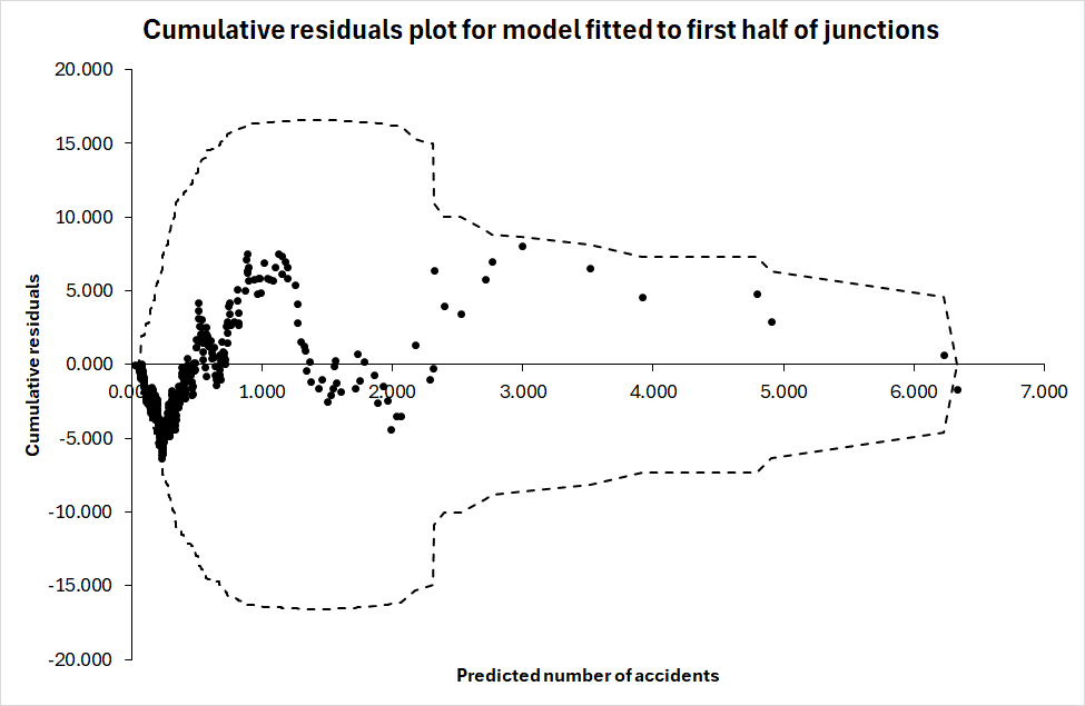
The huge majority of predictions are in the range between 0 and 1. Out of 360 junctions, 296 are predicted to have a lower number of accidents than 1. The predictions between 0 and 1 stray on both sides of the zero residuals line. However, all predictions between 1 and 4 have positive residuals, meaning that in this range the predicted number of accidents is lower than the recorded number of accidents.
It is tempting to think of ways of fixing this. One might, for example, add a square term for entering volume. This would probably shift the predicted values upward in the range between 1 and 4, since the number of accidents depends strongly on traffic volume and this dependence is made stronger by adding a square term. This temptation should be resisted. It is not known if the prediction errors can be attributed to the definition of entering volume or some other variable. It might as well be attributable to one or more omitted variables. Moreover, it affects only 64 of the 360 junctions. Accepting the results of the model fitted without changes, the next questions are: (1) How well does the model predict the number of accidents in the second half of the junctions? (2) How can criteria of falsification of accident prediction models be formulated?
7. A problem of data incompatibility and interpretation
The predictions developed by means of accident prediction models are estimates of the long-term expected number of accidents in each junction. The long-term expected number of accidents is the number of accidents expected to occur per unit of time (in the current data set: six years) if traffic volume (entering vehicles) and risk factors (number of legs, speed limit) remain constant. The data available for empirical testing of the predictions show the recorded number of accidents. This is a whole positive number: 0, 1, 2, etc. The predicted number of accidents, on the other hand, is a continuous variable and can have any positive value: 0.25, 2.43, etc. It is well-known that the recorded number of accidents is not a good estimate of the long-term expected number of accidents but is likely to differ from the expected number of accidents as a result of random variation and/or effects of variables not included in the accident prediction model. How, then, can we determine if predictions are correct – if the data used for this purpose mainly reflect random variation and possibly effects of omitted variables?
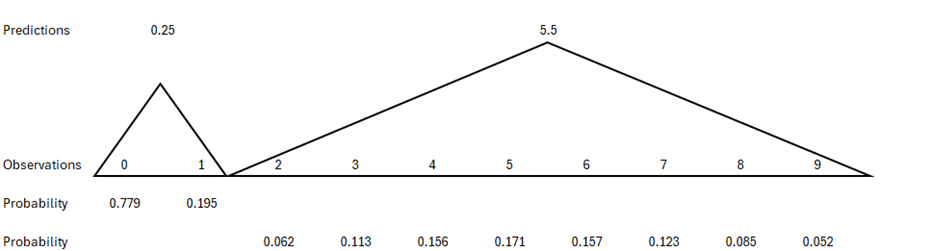
Fortunately, random variation in the number of accidents around a given expected number is known. It is described by the Poisson probability distribution. Therefore, for each predicted number of accidents, the probability for 0,1, etc. accidents to occur is known. This is illustrated in Figure 2.
Figure 2 shows outcomes that can be regarded as consistent with predictions of 0.25 and 5.5 accidents. If the long-term expected number of accidents is 0.25, only the outcomes of 0 and 1 have a probability of 0.05 or more of occurring. If 2 accidents were observed, it would be a very improbable outcome (probability 0.024) – so improbable as to cast doubt on the predicted number. If 5.5 accidents are predicted, the range of outcomes that have a probability of occurring of at least 0.05 is larger, spanning from 2 to 9 accidents. The most probable outcome is 5 accidents, but the probability is not very high (0.171). All outcomes between 3 and 7 have roughly equal probabilities of occurring. Fewer than 2 accidents or more than 9 would be regarded as highly improbable outcomes.
It is now clear that empirical testing of the predictions of a model for each unit of observation must be imprecise in the sense that there is usually no single outcome which is the only one that is consistent with model predictions. For a very low predicted number of accidents, it might be the case that the single outcome of zero accidents has a probability exceeding 0.95. In all other cases, however, several counts of accidents may be viewed as consistent with model predictions. The next section proposes criteria for the falsification of accident prediction models based on this discussion.
8. Falsification criteria for accident prediction models
The basic criterion for assessing whether an accident prediction model is confirmed or rejected by the data is whether the residuals are fully within the scope of random variation or are larger than random variation can account for. More specifically, the following criteria are proposed:
-
The observed number of accidents for each unit of observation should have a probability of at least 0.05 of occurring, given the model-predicted number of accidents. For the whole sample, 95 % should fulfil this criterion.
-
The distribution of accidents in subsamples with a similar predicted number of accidents should not deviate from a random distribution.
-
The residual terms in subsamples with a similar predicted number of accidents should not be greater than random variation can account for.
-
The coefficients for each variable should be consistently replicated when a model is fitted to a data set not known to differ greatly from the data set used to develop predictions.
The use of these criteria is shown in the next section. It should be noted that all four criteria must be satisfied to conclude that a model is supported. If it fails at least one criterion, it is concluded that the model is falsified.
9. Application of falsification criteria
The coefficients estimated in model 4 in Table 2 were applied to predict the number of accidents in the second half of junctions, the 370 junctions that were not used in developing the accident prediction model. These junctions recorded 214 accidents in total; the predicted total number was 236.9. Predictions ranged from a minimum of 0.035 to a maximum of 17.48.
9.1 Consistency of predicted and observed number of accidents
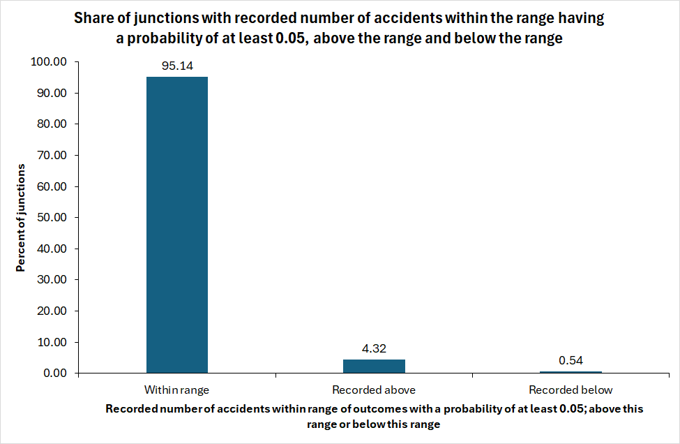
For each predicted number of accidents, the expected distribution of the count of accidents according to a Poisson-distribution having the predicted number of accidents as mean value was computed. Outcomes with a probability of occurrence of at least 0.05 were identified. As an example, in a junction with a predicted number of accidents of 1.626, the probabilities of outcomes were: 0 = 0.197; 1 = 0.320; 2 = 0.260; 3 = 0.141; 4 = 0.057. These outcomes all had a probability of at least 0.05. Hence, any count of accidents between 0 and 4 was regarded as consistent with the prediction. A range of outcomes, each with a probability of at least 0.05, was generated for each of the 370 junctions. The number of outcomes within the range, above the range and below the range was counted. Figure 3 shows the result of the count.
In about 95 % of the junctions, the observed number of accidents was consistent with the predicted number of accidents, i.e. it had a probability of occurring of at least 0.05. In 4.3 % of the junctions, the recorded number of accidents was above the range consistent with the predicted number, and in 0.5 % of the junctions it was below the range consistent with the predicted number. These results show that most predictions were reasonably accurate.
9.2 The distribution of accidents in subsamples
In order to examine the distribution of the recorded number of accidents in subsamples that have a similar predicted number of accidents, the groups listed in Table 4 were formed.
In each group, the Poisson probability distribution of the recorded number of accidents was estimated based on the mean predicted number of accidents. Thus, in the group with a mean of 0.245 (0.20-0.29), the Poisson distribution of the recorded number of accidents between the 43 junctions in this group would be (rounded to the nearest whole number): 34 = 0; 9 = 1. The actual distribution was: 33 = 0; 9 = 1; 1 = 2. When testing the difference between the Poisson-distribution and the actual distribution, cells with expected frequencies (according to the Poisson distribution) lower than 3 were merged to avoid testing involving a very low number of junctions.
| Interval for predicted number of accidents | Number of junctions in group | Mean predicted number of accidents | Mean recorded number of accidents |
|---|---|---|---|
| 0.01-0.09 | 53 | 0.068 | 0.075 |
| 0.10-0.19 | 83 | 0.149 | 0.145 |
| 0.20-0.29 | 43 | 0.245 | 0.256 |
| 0.30-0.39 | 31 | 0.355 | 0.581 |
| 0.40-0.49 | 23 | 0.449 | 0.435 |
| 0.50-0.59 | 17 | 0.540 | 0.588 |
| 0.60-0-69 | 22 | 0.644 | 0.591 |
| 0.70-0.79 | 12 | 0.752 | 0.636 |
| 0.80-0.89 | 15 | 0.858 | 0.933 |
| 0.90-1.09 | 18 | 0.992 | 1.389 |
| 1.10-1.49 | 20 | 1.259 | 1.350 |
| 1.50-1.99 | 14 | 1.749 | 1.143 |
| 2.00- | 20 | 3.851 | 2.350 |
To test if these distributions differ, a Chi-square test was applied. A total of thirteen tests were performed, one for each group listed in Table 4. None of the tests were statistically significant. Hence, the distribution of the accidents in each group did not deviate from the distribution predicted according to the Poisson distribution.
9.3 Residual terms not greater than random
Table 5 shows the assessment of whether the residual terms were greater than random. In the first group, the total predicted number of accidents was 3.608. The recorded number was 4. The residual is 4 – 3.608 = 0.392. The standard error of the residual was estimated as:
\begin{equation*} \text{SE (residual)} = \sqrt{\begin{matrix}Predicted \\ number \ of\\ accidents\end{matrix} \ + \ \begin{matrix}recorded \\ number of \\ accidents\end{matrix}} \end{equation*}This is based on the assumption of a Poisson distribution in which the variance is equal to the mean. Hence, the variance of the predicted number of accidents equals the predicted number of accidents and the variance of the recorded number of accidents equals the recorded number of accidents.
| Interval for predicted number of accidents | Total predicted number of accidents | Total recorded number of accidents | Residual (recorded minus predicted) | Standard error of residual | Ratio of residual to standard error |
|---|---|---|---|---|---|
| 0.01-0.09 | 3.608 | 4 | 0.392 | 2.758 | 0.142 |
| 0.10-0.19 | 12.384 | 12 | -0.384 | 4.934 | -0.078 |
| 0.20-0.29 | 10.530 | 11 | 0.470 | 4.640 | 0.101 |
| 0.30-0.39 | 11.020 | 18 | 6.980 | 5.387 | 1.296 |
| 0.40-0.49 | 10.324 | 10 | -0.324 | 4.508 | -0.072 |
| 0.50-0.59 | 9.181 | 10 | 0.818 | 4.380 | 0.187 |
| 0.60-0-69 | 14.176 | 13 | -1.176 | 5.213 | -0.226 |
| 0.70-0.79 | 8.276 | 7 | -1.276 | 3.908 | -0.327 |
| 0.80-0.89 | 12.867 | 14 | 1.133 | 5.183 | 0.219 |
| 0.90-1.09 | 17.850 | 25 | 7.150 | 6.546 | 1.092 |
| 1.10-1.49 | 25.177 | 27 | 1.823 | 7.223 | 0.252 |
| 1.50-1.99 | 24.485 | 16 | -8.485 | 6.363 | 1.334 |
| 2.00- | 77.010 | 47 | -30.010 | 11.136 | 2.695 |
The residuals are greater than random if the ratio of residuals to the standard error is greater than two or smaller than minus two. As can be seen from Table 4, this was the case in the group where the predicted number of accidents was 2 or more. In this group, the predicted number of accidents was considerably higher than the recorded number. It is concluded that the model fitted to the first half of junctions did not predict the number of accidents correctly when applied to the second half of junctions.
9.4 Replication consistency of coefficient estimates
A negative binomial regression model, identical to the model fitted to the first half of the junctions, was fitted to the second half. The estimated coefficients were compared for the two models. Table 6 shows the comparison.
The differences between the coefficients are the estimate in the first half minus the estimate in the second half. The standard error of the difference was:
\begin{equation*} \text{SE(difference)} = \sqrt{SE_{first \ half}^2 + SE_{second \ half}^2} \end{equation*}| First half | Second half | ||||||
|---|---|---|---|---|---|---|---|
| Term | Estimate | Standard error | Estimate | Standard error | Difference in estimates | SE (difference) | Ratio difference/SE (difference) |
| Constant | -10.9678 | 0.9881 | -10.7634 | 1.1026 | -0.2044 | 1.4806 | -0.1381 |
| Ln(entmaj) | 0.6007 | 0.1069 | 0.7795 | 0.1072 | -0.1788 | 0.1514 | -1.1810 |
| Ln(entmin) | 0.4341 | 0.0799 | 0.2166 | 0.0805 | 0.2175 | 0.1134 | 1.9176 |
| Legs | 0.9710 | 0.2054 | 0.8092 | 0.2365 | 0.1618 | 0.3132 | 0.5165 |
| Dum50 | -0.7273 | 0.2316 | -0.7080 | 0.2773 | -0.0193 | 0.3613 | -0.0534 |
| Dum60 | -0.4155 | 0.2016 | 0.1926 | 0.2070 | -0.6081 | 0.2889 | -2.1045 |
| Dum70 | 0.4649 | 0.2429 | 0.4365 | 0.2534 | 0.0284 | 0.3510 | 0.0809 |
| Dum90 | -0.3030 | 0.5774 | -0.3220 | 0.7609 | 0.0190 | 0.9552 | 0.0199 |
If the ratio of the difference in coefficient estimates to its standard error is greater than two or smaller than minus two, it is interpreted as a systematic difference, greater than pure random variation. As can be seen from Table 6, one of the eight estimated coefficients differed by more than two standard errors. This was the coefficient for the speed limit dummy for a speed limit of 60 km/h. The coefficient for entering volume from the minor road (ln(entermin)) was also close to differing by more than two standard errors.
If consistency in coefficients requires that all coefficients are identical to within random variation, it must be concluded that the requirement is not fulfilled and that the model fitted to the first half of the junctions has not been confirmed for the second half of the junctions. Still, one may ask if the differences in coefficient estimates imply differences in the predicted number of accidents. Figure 4 sheds light on this question. Figure 4 shows the correlation between the predictions based on the model fitted to the first half of the junctions and the predictions on the model fitted to the second half of the junctions.
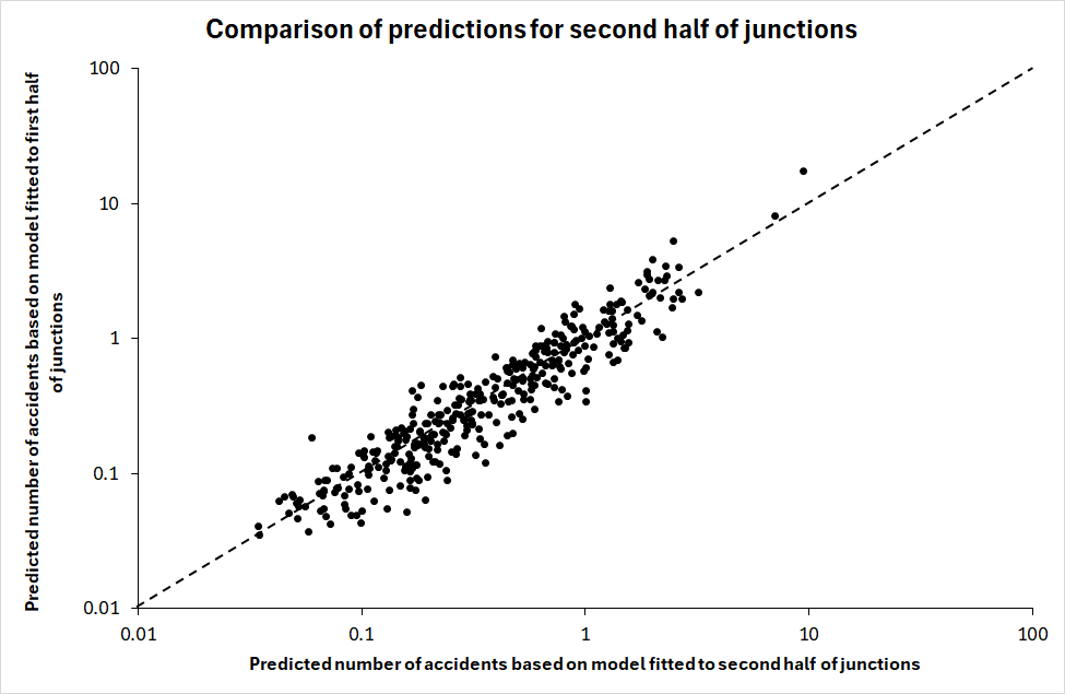
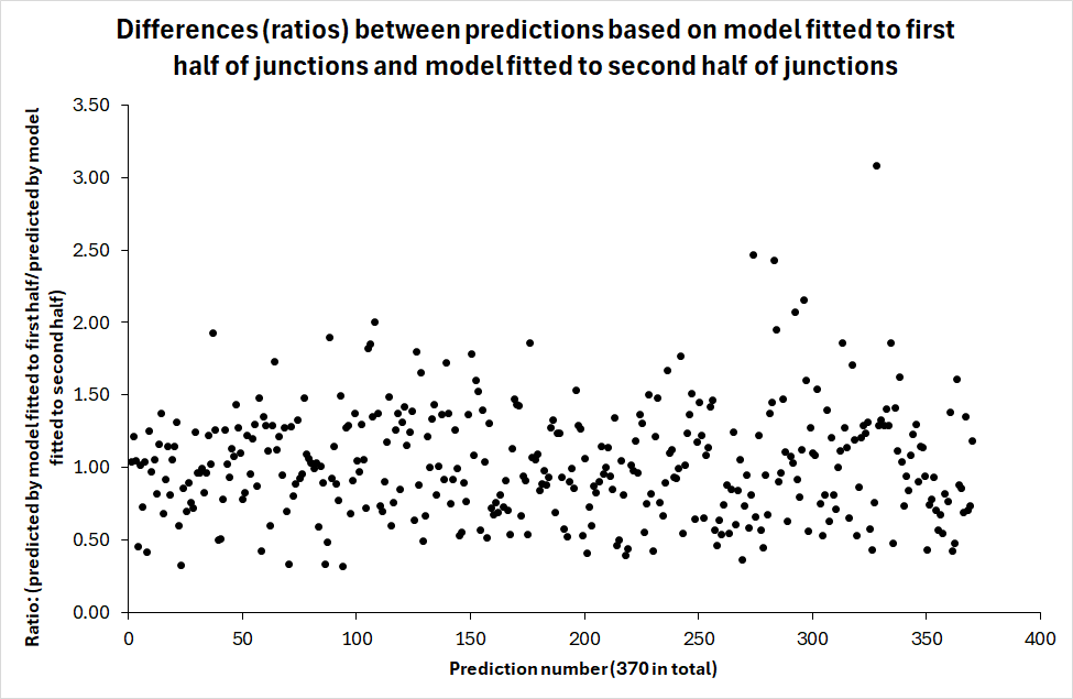
The predictions are correlated (Pearson’s r = .925), but few of them are identical or close to it. If that were the case, all data points would be located on top of dashed 45-degree line showing identical predictions. Figure 5 sheds further light on the differences in the predicted number of accidents. It shows the values of the ratio:
\begin{equation*} \frac{\begin{matrix} Predicted \ number \ of \ accidents according \ to \\ model \ fitted \ to \ first \ half \ of \ junctions \end{matrix}}{\begin{matrix}Predicted \ number \ of \ accidents \ according \ to \\ model \ fitted \ to \ second \ half \ of \ junctions\end{matrix}} \end{equation*}If the predictions were identical, this ratio should have a value of one. Figure 5 shows that very few predictions were identical or close to being so.
It is nevertheless relevant to ask if the differences between the predictions of the two models are larger than random. If the predicted number of accidents for each junction is interpreted as an estimate of the mean value of a Poisson variable, the statistical significance of the differences between the two models in the predicted number of accidents can be tested by estimating the standard error of the difference in predictions as follows:
\begin{equation*} \begin{matrix} \text{Standard error of difference in}\\ \text{predicted number of accidents} \end{matrix} = \sqrt{Pred_1 + Pred_2} \end{equation*}If the difference between two predictions is larger than plus or minus two standard errors, it is statistically significant at the 5 % level. When this test was applied to the two models developed in the paper, not a single difference in the predicted number of accidents was found to be statistically significant. However, many predictions were sufficiently different for the difference to have practical importance, despite its lack of statistical significance.
To give one example, in one junction, the model fitted to the first half of the data predicted 17.5 accidents when applied to the second half of the data. The model fitted to second half of the data predicted 9.4 accidents. The difference, 8.1 accidents, is not statistically significant, given that the predictions are treated as mean values of a Poisson distribution. Yet, one can easily think that the difference would have practical importance. Measures that would be cost-effective if the true long-term expected number of accidents is 17.5 might not be cost-effective if the expected number of accidents is 9.4.
The model fitted to the first half of the junctions explained 94.1 % of the systematic variation in the number of accidents according to the Elvik-index of goodness-of-fit. The model fitted to the second half of the junctions explained 88.2 % of the systematic variation in the number of accidents. Thus, both models had a high explanatory value.
9.5 A preliminary conclusion
A data set consisting of 730 junctions was randomly divided into one group consisting of 360 junctions and one group consisting of 370 junctions. There were no statistically significant differences between the two groups of junctions with respect to:
-
Mean entering volume from the major road
-
Mean entering volume from the minor road
-
Mean number of accidents per junction
-
The relative contributions from random and systematic variation in the number of accidents to the distribution of accidents between junctions
-
The distribution of junctions according to the number of legs (3 or 4)
-
The distribution of junctions with respect to speed limit.
One might expect that an accident prediction model fitted to the first group of junctions could be transferred without modification to the second half of junctions and predict the number of accidents in that group correctly, given that the two groups were so similar. This did not turn out to be the case. Four criteria of falsification were proposed and predictions evaluated with respect to each criterion.
The first two criteria did not indicate that the predictions were systematically wrong. Residual terms were not greater than random variation could account for. The third criterion indicated prediction errors if the predicted number of accidents was more than two. In that case, the model predicted far too many accidents. The fourth criterion – replication of model coefficients – decisively indicated that the model fitted to the first half of junctions was falsified when applied to the second half of junctions. A model was fitted to the second half (370) of the junctions and the coefficients compared to those estimated in the model for the first half of the junctions (360). One of eight estimated coefficients differed systematically (i. e. more than random variation) between the models; a second coefficient was also quite different in value. The predicted number of accidents was different for the two models and was in few cases identical for any of the junctions. The predictions made on the basis of the model fitted to the first half of the junctions were for all junctions different from those based on the model fitted to the second half of the junctions.
All four criteria of falsification must be satisfied to conclude that a model has not been falsified. Since the fourth criterion was clearly not satisfied, and the third only partly satisfied, it is concluded that the model developed for the sample of 360 junctions was falsified when put to the test of predicting the number of accidents in the sample of 370 junctions. This is a very sobering result. When the predictions of a model fail in a sample which is almost identical to the sample used when fitting the model, it is highly unlikely that the predictions would be successful in a different sample. Indeed, it seems likely that any multivariate accident prediction model can only be regarded as a unique statistical description of the data used to fit the model and that it has no predictive validity whatsoever.
10. Discussion
The conclusions stated above may appear to be very discouraging. In fact, they are the opposite. They imply that a new accident prediction model has to be developed in every case knowledge about the long-term expected number of accidents for each unit of observation in a sample is needed. This calls for better data quality and extensive model development. The research needed to serve this end will produce better knowledge of the associations between the number of accidents and factors influencing this number. By contrast, calibration and methods for transfer of accident prediction models do not produce new knowledge. These techniques merely try to bypass the need for developing a new accident prediction model by means of ad hoc adjustments to an existing model.
Accident prediction models should be as parsimonious as possible. The reason for advocating parsimonious models, is that it ought to be a goal of accident modelling to confirm the existence of lawlike relationships between important variables and the number of accidents. One might think that the fact that any accident prediction model is likely to be valid only in the data set it was based on, and that coefficients are likely to vary from model to model, preclude the detection of lawlike relationships. This is wrong. The lawlike relationships are qualitative (or semi-quantitative) and unlikely to ever be quantified precisely. As stated in section 4, the following lawlike relationships are likely to hold for junctions:
L1: The sum of coefficients for entering volume for all legs is greater than 1.
L2: The coefficient for major road entering volume is greater than for minor road entering volume.
L3: The values of the coefficients for entering volume are roughly proportional to the shares (proportions) of traffic entering from the major and minor road but the coefficient for traffic entering from the major road has a smaller value than strict proportionality implies and the coefficient for entering volume from the minor road has a greater value than strict proportionality implies.
L4: There is a safety-in-numbers effect for entering volume from the minor road, implying that the coefficient increases less than in proportion to the share (proportion) of traffic entering from the minor road.
L5: An increase in the number of legs in a junction is associated with an increased number of accidents
L6: Higher speed limits in junctions are associated with a higher number of accidents than lower speed limits
L7: Any design element that adds complexity to a junction is associated with a higher number of accidents.
The existence of these relationships can only be confirmed by numerous replications of studies including an identical set of variables. The findings of studies based on the same set of variables can be synthesised by means of meta-analysis. However, bias may be introduced into meta-analyses of studies not including the same variables. The reason for this, is that the values of the coefficients for the variables different studies have in common are influenced by the inclusion or exclusion of the variables studies do not have in common. This can be seen by comparing the coefficients for traffic volume between models 1-4 in Table 2.
On the other hand, meta-analysis based on models containing the same variables – identically defined and measured can be very informative. The models fitted to the first and second halves of the randomised data set were synthesised and compared to a model fitted to the complete data set. Each coefficient was assigned the following statistical weight:
Statistical weight=1SE2
SE is the standard error of each estimate. Table 7 compares the synthesised coefficients based on meta-analysis with the coefficients estimated for the complete data set.
| Meta-analysis | Model for complete data | ||||||
|---|---|---|---|---|---|---|---|
| Term | Estimate | Standard error | Estimate | Standard error | Difference in estimates | SE (difference) | Ratio difference/SE (difference) |
| Constant | -10.8768 | 0.7359 | -10.9073 | 0.7585 | 0.0305 | 1.0568 | 0.0289 |
| Ln(entmaj) | 0.6898 | 0.0757 | 0.7223 | 0.0762 | -0.0325 | 0.1074 | -0.3021 |
| Ln(entmin) | 0.3262 | 0.0567 | 0.3038 | 0.0565 | 0.0224 | 0.0801 | 0.2794 |
| Legs | 0.9014 | 0.1551 | 0.8618 | 0.1598 | 0.0396 | 0.2227 | 0.1780 |
| Dum50 | -0.7194 | 0.1778 | -0.6811 | 0.1804 | -0.0383 | 0.2533 | -0.1511 |
| Dum60 | -0.1195 | 0.1444 | -0.0657 | 0.1456 | -0.0538 | 0.2051 | -0.2623 |
| Dum70 | 0.4513 | 0.1754 | 0.3929 | 0.1784 | 0.0584 | 0.2501 | 0.2335 |
| Dum90 | -0.3099 | 0.4600 | -0.2018 | 0.4679 | -0.1081 | 0.6561 | -0.1648 |
The synthesised coefficients are very close in value to those estimated for the complete data set. As more data sets are synthesised, the standard errors will become smaller. Formal synthesis of the findings of many studies will drown out the unique characteristics of each data set, which necessitate developing a new model for each new data set. The unique models remain unique to each data set and have a very high probability of falsification if applied to predict the findings of a new data set. This fact, however, does not prevent the development of general knowledge by means of formal research synthesis.
11. Conclusions
The main results of the study presented in this paper can be summarised as follows:
-
Hundreds of accident predictions models have been developed. It is likely that none of them have been tested empirically.
-
To test a model empirically is to use it to predict the number of accidents in an out-of-sample data set, i.e. a different data set from the one used to develop the model.
-
Empirical tests of accident prediction models have a very high probability of falsification of the models. This reflects the fact that any model is only a sample-specific statistical description of the data set it has been fitted to.
-
No accident prediction model is likely to be valid for any other data set than the one it was fitted to. Methods for calibration and model transfer cannot eliminate the need for developing a new model for each new data set.
-
The fact that models are unique to each data set does not prevent developing general knowledge of the relationships between the number of accidents and variables influencing the number of accidents. Meta-analysis of models based on the same set of variables is an effective tool for developing general knowledge.
Declaration of conflict of interest
The author declares that he has no known competing financial interests or personal relationships that could have appeared to influence the work reported in this paper.
CRediT contribution statement
Rune Elvik: Conceptualization, Formal analysis, Writing—original draft, Writing—review & editing.
Ethics statement
The research reported in this paper did not involve human subjects and did not require ethical approval.
Use of artifical intelligence
No AI tools were used in writing this paper or in performing the analyses reported in it.
Funding
This study did not receive any funding.
Editorial information
Handling editor: Stijn Daniels, Transport & Mobility Leuven, Belgium | KU Leuven, Belgium.
Reviewers: Bhagwant Persaud, Toronto Metropolitan University, Canada; Akis Theofilatos, University of Thessaly, Greece.
Submitted: 11 July 2025; Accepted: 7 January 2026; Published: 20 January 2026.