Lateral shifting behavior of vehicles at horizontal curves and its influencing factors: application of LightGBM and SHAP
Abstract
Horizontal curves are disproportionately associated with severe crashes due to increased vehicle instability and lane departure risks. This issue is particularly critical in low- and middle-income countries (LMICs), where poor lane discipline, mixed traffic, and geometric inconsistencies amplify crash potential. Despite its significance, lateral shifting (LS) behavior on horizontal curves remains understudied in LMIC contexts. This study addresses the research question: What are the key factors influencing the lateral shifting behavior of vehicles on rural horizontal curves, and how can they be modeled and interpreted effectively in LMIC conditions? Using trajectory data from 8,748 vehicles across 18 curve segments in India, an explainable machine learning framework is developed. Light Gradient Boosting Machine (LightGBM) was selected for its superior performance in classification metrics compared to other ML models. SHapley Additive exPlanations (SHAP) were integrated to interpret model outputs and quantify feature contributions, while Shannon entropy was applied to assess prediction uncertainty. Findings reveal that lane type, vehicle speed, curve radius, lateral clearance, superelevation, and traffic interactions, especially oncoming vehicles, significantly influence lateral shifting behavior. SHAP analysis uncovers nonlinear effects and interaction patterns, including a threshold response to speed and clearance. Notably, the influence of preceding vehicles differs from oncoming traffic, suggesting asymmetric behavioral responses rarely captured in prior studies. This research fills four major gaps in existing literature related to context, terrain, feature scope, and methodology. It provides data-driven insights to support safer curve design and lane departure countermeasures tailored to LMIC road environments.
1. Introduction
1.1 Risk at horizontal curve
Road crashes are, unfortunately, one of the leading causes of death globally, resulting in 1.19 million fatalities each year (WHO, 2023). As per the European Commission (2021), the curved segments are considered to be more prone to fatal crashes than straight-road segments. For example, crash risk on curved segments is found to be 1.5 to 4 times higher than on straight road segments (Alexei et al., 2005; Chakraborty & Gates, 2023; Wu & Xu, 2017). The Indian Ministry of Road Transport & Highways (MoRTH, 2022) reported that out of 168,491 annual road fatalities, a significant number of 20,573 occurred at horizontal curves, making them the second-highest contributor to total road deaths in India. Further, past studies have clearly reported that crash severity is higher on sharp curves with radii less than 100 m (Awasthi et al., 2024; Schneider et al., 2009; Xin et al., 2017). As per the National Highway Traffic Safety Administration (NHTSA, 2016), negotiating the horizontal curve is one of the riskiest maneuvers and the second-highest contributor to single-vehicle and two-vehicle fatal crashes in the United States. This elevated crash risk is often linked to a combination of complex geometric road alignments and driver-related factors such as inadequate speed adjustment, misjudgment of curve sharpness, and difficulty in maintaining appropriate lateral position during curve navigation (Hallmark, 2012). These challenges often lead to higher crash frequencies and severities. This pattern is evident in targeted safety programs like SAFESTAR. The program classifies curves by risk and shows that appropriately treating high-risk curves, such as through speed management measures or horizontal and vertical signing, can significantly reduce crashes (Cafiso et al., 2019). Although crash statistics provide essential historical evidence for understanding roadway safety, analyzing the lateral positioning behavior of vehicles while negotiating a curve is equally crucial for understanding how crash risk can develop even at locations with no prior crash history.
1.2 Background
Understanding how vehicles behave while negotiating horizontal curves has been an important concern in transportation safety research for decades. Horizontal curves require drivers to adapt to dynamic geometric demands, such as changes in alignment and visibility. Misalignment between vehicle LP and curve design can result in run-off-road or head-on crashes. Several past studies have explored the role of road geometry, speed, and signage in shaping vehicle paths at curves. Early empirical field studies formed the backbone of the understanding of lateral position behavior on curves. An early study by Glennon & Weaver (1971) used photographic tracking of over 500 vehicles across five rural Texas curves to highlight significant deviations between actual vehicle paths and those assumed in highway design. They found that a noticeable portion of vehicles followed paths that were much sharper than what the curve was originally designed for, highlighting that relying only on geometric design assumptions does not fully reflect how drivers actually behave on the road. It offered a percentile-based rationale for path design but lacked behavioral nuance and contextual adaptation. However, as an early study, it was understandably limited to passenger vehicles.
Subsequent studies refined the understanding of how lateral positioning is influenced by operational features and visual cues. Krammes & Tyer (1991) conducted a before–after study comparing post-mounted delineators with retroreflective raised pavement markers (RPMs) on rural curves in Texas. Their findings indicated that RPMs improved lane adherence and reduced centerline encroachments. However, data were collected only at night, limiting the applicability of findings to daytime driving conditions. Similarly, Hallmark (2012) utilized pneumatic road tubes to record speeds and lateral positions on three rural curves in Iowa, USA. By analyzing the odds of lane-edge encroachment for vehicles exceeding the advisory speed, a strong association between speed and lateral deviation was observed. Despite its pragmatic outcome, the limited study locations and vehicular uniformity constrained its relevance beyond controlled, homogeneous traffic environments.
To better understand lateral dynamics under complex spatial and perceptual conditions, researchers adopted simulation-based approaches. Charlton (2007) used a high-fidelity simulator to test driver reactions to various curve treatments, including chevrons, rumble strips, and herringbone markings. His results showed that while conventional warning signs were ineffective in reducing speed or improving lane positioning, treatments like rumble strips and chevrons significantly enhanced lateral control, especially on sharper curves. Bella (2013) expanded on this by assessing how roadside features such as trees and guardrails affect lateral positioning and perceived safety. The study found that while guardrails increased lateral deviation in some configurations, the presence of trees had minimal impact on behavior, despite an elevated risk. Mauriello et al. (2018) conducted a driving simulator study on two-lane rural highways using 50 drivers' lateral deviation across eight curves. The study found that sharp curves resulted in higher lateral deviations and more frequent lane departures. Bassani et al. (2019) tested how drivers compensate for sight distance limitations in curves. Using detailed geometric modeling and a driving simulator, they observed that drivers tend to reduce their speed when faced with obstructed views. Though behaviorally insightful, simulation-based findings are limited by their inability to capture real-world distractions and mixed traffic complexity.
In contrast to these controlled studies, few researchers have pursued more data-rich, behaviorally grounded approaches. Fitzsimmons et al. (2013) collected over 23,000 vehicle trajectories using pneumatic tubes along urban and rural curves in Iowa, USA. Using linear mixed-effects models, they linked entry speed and vehicle type to lateral position, revealing that motorcycles and passenger cars exhibited more pronounced centerline encroachment than larger vehicles. While methodologically strong, the study excluded basic geometric factors such as curve radius and length, which reduces its applicability to regions where road geometry is a primary safety concern. Similarly, Havránek et al. (2020) employed a before–after design to assess how road markings influence lateral behavior on rural Czech roads. Their findings showed that centerlines generally pushed drivers away from the centerline, whereas edgelines sometimes caused shifts toward the center. Some studies have attempted to classify actual vehicle paths on curves using trajectory tracking. Maljković & Cvitanić (2016) studied path radii in Croatia using GPS-equipped vehicles and found that actual trajectories were typically tighter than the design curve radius. Among the few studies from Low and Middle-Income Countries (LMICs) contexts, one of the earliest was by Das et al. (2016), who used manual data collection at eight locations and found that commercial vehicles exhibited higher lateral deviations compared to passenger cars. A consolidated summary of these studies, covering diverse methods and influencing factors, is given in Table 1.
| Study | Country | Road type | Method | Key factors influencing lateral shifting behavior |
|---|---|---|---|---|
| Glennon and Weaver (1971) | United States | 2L-U | Video-based; Linear regression | Curve radius (−), Superelevation (−) |
| Krammes and Tyer (1991) | United States | 2L-U | Sensor-based; Traditional hypothesis testing | RPMs caused vehicles to stay away from the centerline |
| Charlton (2007) | New Zealand | 2L-U | Driving simulator; Traditional hypothesis testing | Herringbone marking (–), Chevron signs (–), Curve radius (–) |
| Stodart et al. (2008) | United States | 2L-U | Instrumented vehicle data; Linear-regression, | Curve radius (–), Speed (+), Average grade ≥5% (–) |
| Ben-Bassat and Shinar (2011) | Israel | Divided four-lane | Driving simulator; Traditional hypothesis testing | Guardrail (–), Curve radius (–) |
| Hallmark (2012) | United States | 2L-U | Sensor-based; odds ratio | Speed (+) |
| Bella (2013) | Italy | 2L-U | Driving simulator; Multivariate hypothesis testing | Guardrail (+) |
| Fitzsimmons et al. (2013) | United States | 2L-U | Sensor-based; Linear Mixed-Effects Model | 2W and Car (+), Nighttime (+), Outer lane vehicles (+), Speed (+), Curve length (–) |
| Das et al. (2016) | India | 2L-U | Manual field observation using marked strips; Descriptive statistics | Curve radius (–), Carriageway width (+), Heavy vehicle (+) |
| Maljković & Cvitanić (2016) | Croatia | 2L-U | Instrumented vehicle data; Multiple Linear Regression | Curve radius (–) |
| Mauriello and Domenichini (2018) | Italy | 2L-U | Driving simulator; Categorical hypothesis testing | Curve radius (–), Correcting behavior (+) |
| Bassani et al. (2019) | Italy | 2L-U | Driving simulator; Traditional hypothesis testing | Curve radius (–), Sight obstruction distance from road edge (–), Visibility condition (–) |
| Havránek et al. (2020) | Czech Republic | 2L-U | Video-based; Non-parametric hypothesis testing | Only edgeline present (+), Only centerline present (–) |
Recent safety research highlights that proactive crash risk assessment depends strongly on how proactive risk assessment is important and is conceptualized, and how data are structured for reliable modeling across sites (Cafiso et al., 2018; Chen et al., 2025; Yastremska-Kravchenko et al., 2022). In line with this paradigm, the present study develops an explainable, data-driven framework that links individual vehicle LP and lateral shifting behavior to interpretable indicators of lane departure risk on two-lane, undivided horizontal curves.
1.3 Research gaps and objectives
Collectively, past studies have advanced the understanding of lateral shifting behavior across diverse traffic and road-geometric environments. However, most field studies and models are limited to high-income countries, rely on simulations, use only statistical methods for interpretation, or consider an incomplete set of factors. There is an absence of studies that simultaneously consider vehicle type, traffic interaction, curve geometry, infrastructure features, and visibility in a unified framework, especially on hilly horizontal curves, where obstructed visibility and heterogeneous traffic demand for a fundamentally different lens for analysis. Further, the weak lane discipline and the heterogeneity of traffic in LMICs add further complexities in analyzing this lateral shifting behavior (Debbarma et al., 2025; Tiwari et al., 2000; Trivedi & Gor, 2017).
The present study aims to address these gaps by (i) employing a machine learning algorithm to model the lateral shifting behavior of vehicles and (ii) identifying the key factors and their influencing patterns on the lateral shifting behavior at hilly horizontal curves. To achieve this, the study adopts a data-driven approach where naturalistic data were collected at 18 sharp horizontal curves across four northeastern hilly states of India, incorporating an extensive set of 15 factors. These include standard geometric and traffic variables, as well as less explored parameters such as curve length, longitudinal grade, lateral clearance, presence of oncoming or preceding vehicles, presence of curve ahead sign, and diverse vehicle types. The study incorporates a diverse range of vehicle types typical of Indian mixed traffic, namely two-wheelers (2W), cars, sport utility vehicles (SUVs), light commercial vehicles (LCVs), and heavy vehicles (HVs), to capture the effects of different vehicle sizes while negotiating a curve, a critical aspect that has been largely overlooked in prior research. Furthermore, this study employed Light Gradient Boosting Machine (LightGBM) (Ke et al., 2017), a robust machine learning technique, to model a comprehensive set of factors influencing lateral shifting behavior. To overcome the common challenge of interpretability in ML models, SHapley Additive exPlanations (SHAP) was subsequently applied to effectively quantify the contribution of each factor, ensuring both predictive accuracy and analytical transparency (Guo et al., 2022; Shapley, 1953). The remainder of the paper is organized as follows: Section 2 presents the methodology, Section 3 describes the data collection and extraction process, Section 4 discusses the model results and their interpretation, Section 5 highlights the key findings, and Section 6 concludes the study.
2. Methodology
As discussed earlier, past studies in this area predominantly relied on traditional statistical methods (Table 1). While these methods are useful for identifying general trends, they often require strict assumptions (e.g., linearity) and struggle to capture complex nonlinear interactions across diverse influencing factors. In contrast, modern ML techniques offer greater flexibility by learning patterns directly from data without the need to specify a predefined functional form. This capability makes ML methods particularly effective for modeling the complex vehicular dynamics and driver behavior, which has led to their growing adoption in traffic safety research (Wen et al., 2021).
Given these advantages, the present study employs LightGBM, a gradient boosting decision tree (GBDT) algorithm, to model vehicle lateral shifting along horizontal curves. LightGBM has gained wide acceptance due to its computational efficiency, scalability, and high predictive accuracy across a range of domains (Jalal et al., 2024). It is particularly well-suited for binary classification problems, as in our case, and has been shown to outperform traditional statistical models and other ML algorithms, such as logistic regression and Support Vector Machines (Ponsam et al., 2021). When compared to other gradient boosting frameworks such as XGBoost, LightGBM offers several key advantages. It adopts a leaf-wise tree growth strategy and histogram-based decision splitting, which substantially improves training speed, without compromising model accuracy (Jalal et al., 2024; Ke et al., 2017). This makes it ideal for large datasets or real-time applications where computational efficiency is critical (Jalal et al., 2024). Additionally, LightGBM handles categorical features natively, allowing direct splits on category equality without resorting to one-hot encoding, which can increase model complexity (Hancock & Khoshgoftaar, 2020). Therefore, the present study employs LightGBM as the primary modeling tool, given its proven capability to handle a wide range of continuous and categorical variables effectively in binary classification tasks.
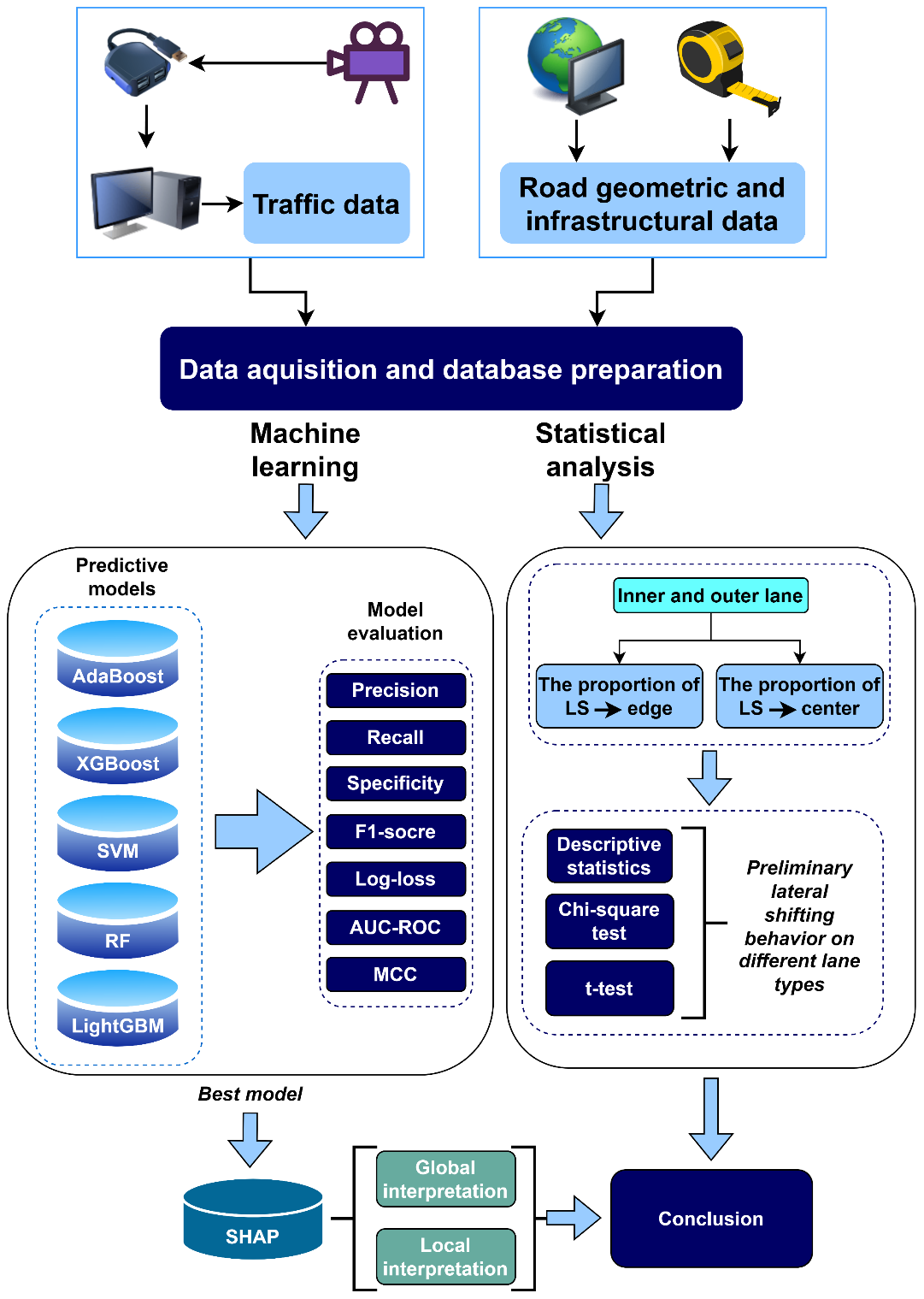
However, like many other ML techniques, LightGBM suffers from a key drawback: its black-box nature, which makes it difficult to interpret how input variables contribute to model predictions. To overcome this limitation, the present study employs the SHapley Additive exPlanations (SHAP), a model interpretability tool that attributes each prediction to individual input variables. SHAP summary plots reveal the most influential variables and their direction of impact, while dependence plots illustrate how changes in a specific variable influence the output, including its interaction with other variables. This approach enhances the interpretability of the LightGBM model, making it more transparent and easier to understand. A detailed flowchart of the study is provided in Figure 1. Additionally, Shannon’s Entropy is incorporated to measure the uncertainty in prediction probability. This helps in assessing the reliability of the model’s outputs and provides insights into the variability in lateral shifting behavior. The following subsections provide a concise overview of the concept of lateral shift used in the study, LightGBM, SHAP, and Shannon’s Entropy. Further details on these methodologies can be found in (Ke et al., 2017; Lundberg & Lee, 2017; Mosca et al., 2022; Shannon, 1948).
2.1 Concept of lateral shift
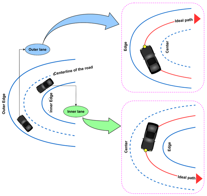
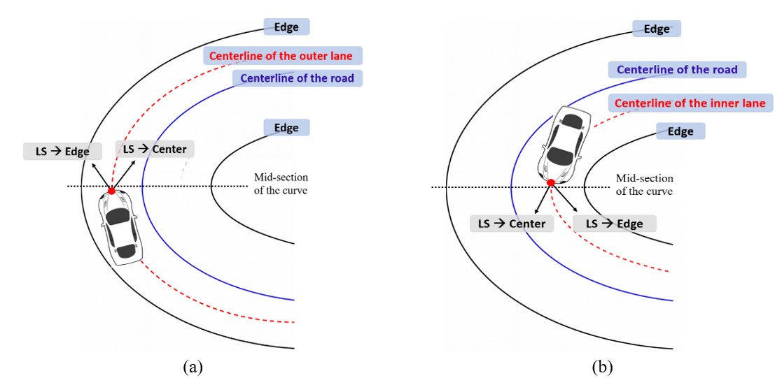
According to Spacek (2005), a vehicle is considered to be following the ideal path when the lateral position of the front of the vehicle aligns with the center of the lane (inner or outer) while maneuvering a horizontal curve. Figure 2 illustrates a two-way, two-lane undivided horizontal curve, where the blue dotted line represents the centerline of the road, the red lines indicate the centerline of each lane, and the yellow circle marks the lateral position of vehicles. If the carriageway width (CW) is used as a reference, the centerline of the road is located at 0.5CW, while the centerlines of individual lanes are positioned at 0.25CW from their respective edges. However, when the LP of a vehicle deviates from this ideal path, a Lateral Shift (LS) is observed. Within any given lane, an LP within the range of 0 to 0.25CW is classified as a shift toward the edge, whereas an LP exceeding 0.25CW is considered a shift toward the centerline of the road.
2.2 Light gradient boosting machine
LightGBM, developed by Microsoft and Peking University (Ke et al., 2017), is a gradient-boosting method designed to efficiently handle high-dimensional datasets. It improves upon traditional Gradient Boosting Decision Trees (GBDT) and eXtreme Gradient Boosting (XGBoost) by incorporating Gradient-based One-Side Sampling (GOSS) and Exclusive Feature Bundling (EFB). These advancements enable LightGBM to achieve faster training times while maintaining high predictive accuracy.
If the dataset used for training consists of independent variables {x1, x2, …, xn} and a dependent variable y. Then, the predicted value of GBDT is given by Equation (1).
\begin{equation} f(x) = \sum_{t = 1}^{T}{h_{t}(x)}\tag{1} \end{equation}where ht(x) denotes the outputs of decision tree models and T is the number of trees in the model. In this context, the approximation function \(\widehat{f}\) that optimally minimizes the loss function L(y, f(x)) is given by Equation (2)
\begin{equation} \widehat{f} = {\arg\min}_{f}E_{y,\ \ S}L(y,f(x))\tag{2} \end{equation}Ey,s denotes the expected loss over the joint distribution of true labels 𝑦 and input samples 𝑠. Unlike traditional GBDT, which splits internal nodes based on information gain, LightGBM employs the GOSS method for node splitting. This approach prioritizes samples with high gradient magnitudes by selecting the top \([a \times 100\%]\) of instances with the largest absolute gradients as subset A. Meanwhile, a proportion \([b(1 - a) \times 100\%]\) of the remaining lower-gradient samples are randomly sampled to form subset B. The final node split is then determined by maximizing the variance gain Vj(d) over the combined subset A∪B using Equation (3).
\begin{eqnarray} V_{j}(d) = \frac{1}{n}\left\lbrack\frac{{(\sum_{x_{i} \in A_{l}}^{}{g_{i} + \frac{1 - a}{b}}\sum_{x_{i} \in B_{l}}^{}g_{i})}^{2}}{n_{l}^{j}(d)} + \frac{{(\sum_{x_{i} \in A_{r}}^{}{g_{i} + \frac{1 - a}{b}}\sum_{x_{i} \in B_{r}}^{}g_{i})}^{2}}{n_{r}^{j}(d)}\right\rbrack\tag{3} \end{eqnarray}where gi represents the negative gradient of the loss function at each iteration, and Al = {xi ∈ A : xij ≤ d}, Ar = {xi ∈ A : xij > d}, Bl = {xi ∈ B : xij ≤ d}, Br = {xi ∈ B : xij > d}. Furthermore, LightGBM enhances training speed using the EFB technique, which groups mutually exclusive sparse features to minimize unnecessary splits and computations. Additionally, a feature scanning algorithm optimizes histogram construction, enabling efficient processing of high-dimensional datasets without compromising accuracy. It also handles multicollinearity, making it ideal for applications like traffic safety analysis (Xue et al., 2024; Zhang et al., 2023). By integrating GOSS to prioritize important data and EFB to reduce feature complexity, LightGBM enhances training efficiency and predictive performance, excelling in handling large-scale, sparse datasets while maintaining high accuracy and computational efficiency.
Figure 3 presents a flowchart depicting the general architectural workflow of LightGBM.

The process begins with inputting the dataset, which includes multiple influencing factors and a binary target variable. The data is then split into a training and a testing set. To ensure reliable model performance, cross-validation is performed on the training set, allowing the model to be trained and validated on different data partitions.
The core modeling phase involves LightGBM, a gradient boosting algorithm optimized for decision tree-based learning. During training, the model initializes a base prediction and iteratively updates it using gradient information. It employs Gradient-based One-Side Sampling (GOSS) to focus on high-impact samples and Exclusive Feature Bundling (EFB) to reduce feature dimensionality. Leaf-wise trees are constructed using histogram-based splitting to maximize learning efficiency.
The training continues until a predefined stopping criterion is met, such as a maximum number of iterations or the maximum tolerable error is achieved. After cross-validation, the model is retrained on the entire training data and then tested on a separate hold-out set to check how well it performs on a new dataset. This structured process ensures model robustness, interpretability, and readiness for SHAP-based analysis.
2.3 Shapley additive exPlanations
Interpreting machine learning (ML) models is a crucial challenge, particularly in traffic safety research, where many studies have primarily focused on enhancing predictive accuracy and comparing model performances. However, understanding the influence of various influencing factors and their combined effects is equally important for guiding safety interventions. SHAP (SHapley Additive exPlanations) is a powerful interpretability method based on Shapley values from statistical game theory, which allows for an optimal distribution of feature contributions while providing local interpretability (Ding et al., 2024; Lundberg & Lee, 2017; Wen et al., 2021). SHAP can be applied to various ML models to analyze and explain their predictions.
For a given subset of influencing factors S⊆F (where F represents the entire set of influencing factors), two models are trained, one that includes factor i, denoted as fS∪{i}(xS∪{i}) and another that excludes it, fS(xS). Here, xS∪{i} and xS correspond to the input values with and without factor ‘i', respectively. The Shapley value of an influencing factor ‘i’ is calculated using Equation (4) (Shapley, 1953).
\begin{eqnarray} \varnothing_{i} = \sum_{S \subseteq F\backslash\text{\{}i\}}^{}\frac{|S|!\left( |F| - |S| - 1 \right)!}{|F|!} (f_{S \cup \left\{ i \right\}}(x_{S \cup \left\{ i \right\}}) - f_{S}(x_{S}))\tag{4} \end{eqnarray}However, Equation (4) becomes computationally expensive as the number of features increases, leading to exponential growth in complexity. To address this issue, Lundberg et al. (2020) introduced a computationally efficient method called TreeExplainer, specifically designed for decision tree-based ensemble machine learning (EML) models like LightGBM. This approach significantly enhances the efficiency of calculating SHAP values at both local and global levels (Ayoub et al., 2021). Local SHAP values measure the impact of features for a single observation, whereas global SHAP values evaluate overall feature importance and interactions between influencing factors across the dataset. The SHAP interaction values, which quantify how two factors jointly influence predictions, can be calculated using Equation (5).
\begin{eqnarray} \varnothing_{i,j} &=& \sum_{S \subseteq F\backslash\text{\{}i,j\}}^{}\frac{|S|!\left( |F| - |S| - 2 \right)!}{|F|!}(f_{S \cup \left\{ i,j \right\}}\left( x_{S \cup \left\{ i,j \right\}} \right) - f_{S \cup \left\{ i \right\}}\left( x_{S \cup \left\{ i \right\}} \right)\nonumber\\ && - f_{S \cup \left\{ j \right\}}\left( x_{S \cup \left\{ j \right\}} \right) + f_{S}(x_{S}))\tag{5} \end{eqnarray}This research employs LightGBM to model vehicle lateral shifting behavior at horizontal curves, aiming to identify and quantify the most influential factors contributing to this phenomenon. The objective is to enhance understanding and support the development of targeted safety countermeasures. To assess the effectiveness of the proposed approach, the LightGBM model is compared against several widely used machine learning algorithms, including AdaBoost, Random Forest, Support Vector Machine (SVM), and XGBoost. Furthermore, the SHAP method is utilized to analyze the LightGBM results, providing a comprehensive evaluation of critical factors influencing lateral shifting behavior.
2.4 Shannon’s entropy method
Shannon entropy, introduced by Claude Shannon (Shannon, 1948) in communication theory, is a fundamental measure of uncertainty in probability distributions. It quantifies the degree of disorder or unpredictability in a system, making it widely used for assessing uncertainty in classification models. For a classification problem where a model predicts probabilities for multiple classes, entropy is computed using Equation (6).
\begin{equation} H(P) = - \sum_{i = 1}^{n}{p_{i}\log_{2}p_{i}}\tag{6} \end{equation}where pi represents the predicted probability of a sample belonging to class i, and n is the total number of classes. Shannon entropy ranges from 0 to log2 n, where higher entropy values indicate uncertain predictions where the model struggles to make a clear decision, whereas lower entropy values suggest strong confidence in classification. In this study, Shannon entropy has been applied to quantify the uncertainty in LightGBM’s predicted probabilities. By computing entropy for each predicted probability, the model's confidence and uncertainty in classifications are assessed.
3. Data
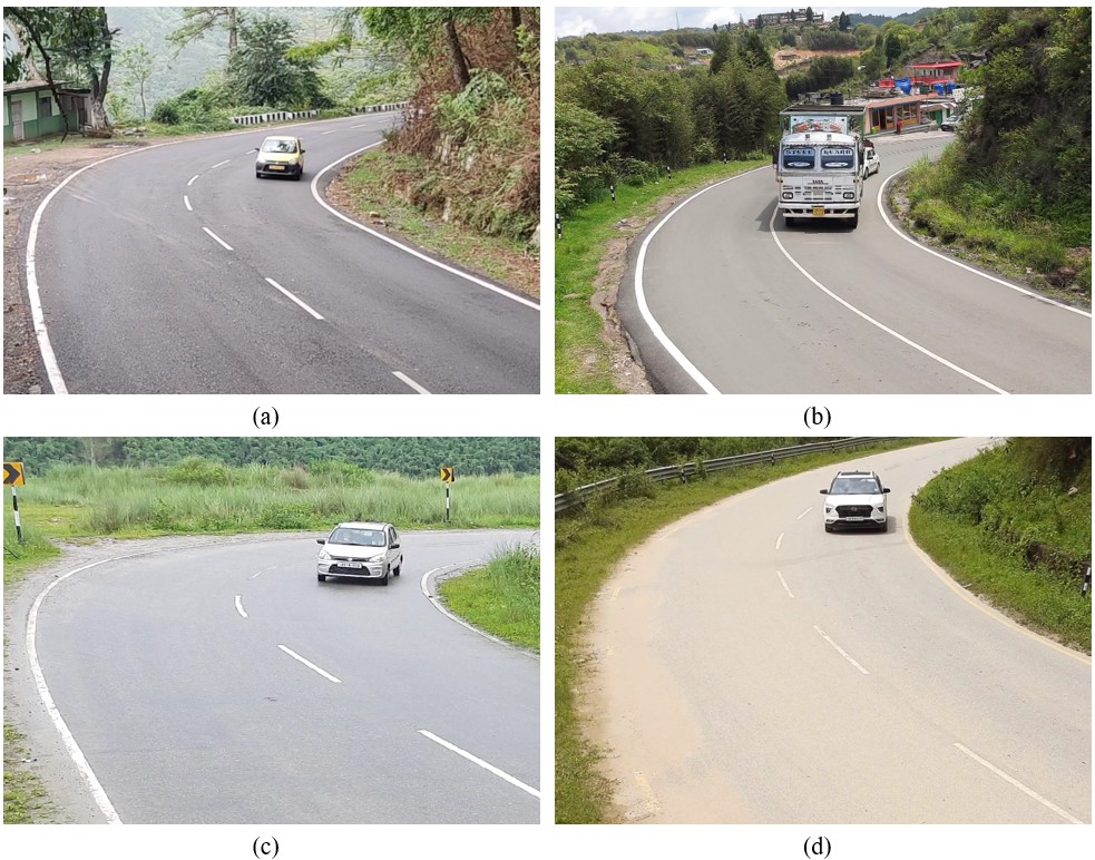
The dataset used in this study was collected by videography along with a manual on-site survey on 18 distinct horizontal curves across four different states in India, viz. Arunachal Pradesh, Meghalaya, Mizoram, and Nagaland. These states are situated in the country's northeast region, characterized by hilly terrain with a high prevalence of horizontal curves. Figure 4 presents representative snapshots from the video recordings of various horizontal curves.
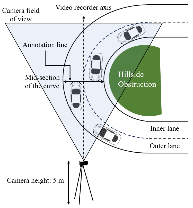
All locations are situated along rural hilly highways connecting inter-urban areas. The video data was collected under dry weather conditions and during daylight hours to minimize the potential influence of adverse weather on vehicle behavior and visibility. The dataset comprises a comprehensive set of design variables that are anticipated to influence vehicle lateral shifting behavior, incorporating traffic-related, geometric, and infrastructural factors. To ensure the accuracy of the Lateral Shift data, a video recorder was mounted on the top of a 5 m tall camera stand in such a way that its line of axis could be perpendicular to the annotation line made virtually at the middle of the curve, as shown in Figure 5. Although the challenging hilly terrain did not always permit a perfectly perpendicular setup, the camera position was set up in a way that limited the yaw angle to < 5° at all sites. Within this range, any possible error in lateral position is minimal (< 2%) and is not expected to affect the results.
The primary reason for this particular camera configuration was to obtain a clear, unobstructed top-down view of the entire curve segment, thereby minimizing sidewise measurement errors during manual extraction of LP. Using this camera setup, video recordings were conducted for 2 hours at each curve location, with data collected on a separate weekday for each curve. These recordings were later played on a computer screen, and a total of 8,748 lateral position (LP) data points were extracted for both outer and inner lanes, using the Kinovea software (a video annotation software).
The lateral position (LP) and lateral shift (LS) of vehicles were deliberately calculated at the curve’s mid-section, as previous studies have shown that the maximum lateral deviation typically occurs at this location (Debbarma & Biswas, 2024; Fitzsimmons et al., 2013). To collect the LP of vehicles, the curve’s mid-section was identified by first marking the start and end of the horizontal curve in the field using the manual line-of-sight method. These endpoints were validated using AutoCAD’s geolocation feature with satellite imagery, and the curve's mid-section was marked. In the Kinovea software, an annotated reference line was then placed at the mid-section of the curve and calibrated using the field-measured carriageway width (say, 7.5 m), as shown in Figure 6a. The LP values for both front wheels were recorded (say, 5.61 and 6.85 m), as shown in Figure 6a, and their average was computed to determine the vehicle's central LP (6.23 m). For two-wheelers (2W), which have a single front wheel along the center axis, its LP was directly taken as the vehicle’s midpoint. This procedure is consistent with previous studies (Bhavna & Biswas, 2022; Saini & Biswas, 2021; Sharma et al., 2025). To complete the data extraction within a reasonable timeframe, two individuals were involved in the process. This helped speed up the extraction while maintaining consistency and accuracy.
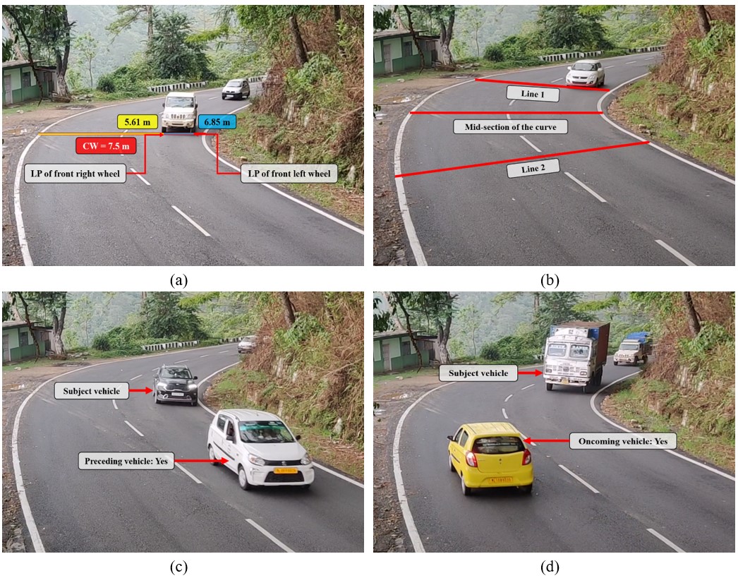
To measure vehicle speed, two additional lines, line 1 and line 2, were drawn 15 m before and after the midpoint line, creating a total distance of 30 m. The amount of time a vehicle’s front took to cover the distance between these lines was recorded to estimate the speed \(\left(Speed = \frac{Curved \ distance \ travelled}{Time \ elapsed}\right)\), as illustrated in Figure 6b. The data related to the curved distance travelled and time elapsed of individual vehicles was fetched from the Kinovea video annotation software. Information regarding the presence of preceding and oncoming vehicles was manually verified from the video, as seen in Figure 6c–d. Subsequently, these data were organized by lane type. Vehicles were categorized manually from the footage into five types based on their size: two-wheelers (2W), standard cars (Car), sport utility vehicles (SUV), light commercial vehicles (LCV), and heavy vehicles (HV). Table 2 presents the details on traffic volume, vehicle composition, and speed distribution.
| Parameter | Inner lane | Outer lane | |
|---|---|---|---|
| Traffic volume (veh/hr) | 163–349 | 195–377 | |
| Vehicle proportion (%) | 2W | 23–37 | 23–41 |
| Car | 18–26 | 16–28 | |
| SUV | 16–22 | 17–23 | |
| LCV | 10–19 | 9–18 | |
| HV | 7–18 | 9–20 | |
| Traffic Speed (km/hr) | Minimum | 15 | 15 |
| Maximum | 75 | 74 | |
| Mean | 39 | 37 | |
| 85th percentile | 47 | 44 | |
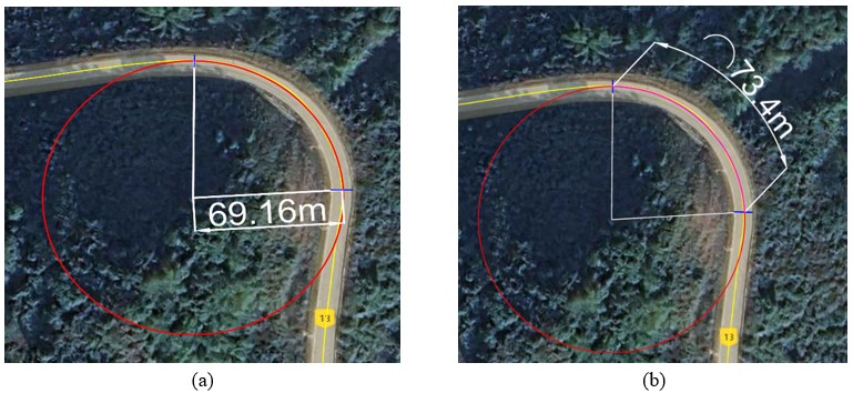
Geometric factors, such as curve radius, were measured using AutoCAD’s geolocation tool, as illustrated in Figure 7a, to ensure high accuracy. The curve length was initially measured in the field along the centerline from the curve’s entry to its exit and subsequently verified using AutoCAD’s geolocation tool, as shown in Figure 7b. The variation in curve length was observed to fall within the acceptable range of ±2 to ±7 meters, depending on the curve radius (25–100 m).
Subsequently, superelevation, longitudinal grade, lateral clearance, shoulder width, and the presence of speed limit signs, chevron signs, and curve ahead signs were manually recorded through an on-site survey. The outcome variable, lateral shift (LS), was derived from the central lateral position (LP) of vehicles, as previously discussed in subsection 2.1 and further illustrated in Figure 8.
A detailed description of all variables is provided in Table 3. Following data cleaning and the removal of erroneous entries, the final dataset comprises 8,748 vehicles along with their corresponding LP data. The observed vehicle categories are motorized two-wheelers (15.90%), cars (46.08%), sport utility vehicles (25.30%), light commercial vehicles (6.65%), and heavy vehicles (6.07%). The study aims to analyze the effects of various influencing factors on LS. To facilitate model development and evaluation, the dataset was partitioned into training and testing subsets using a 70–30 split.
| Variable | Description | Mean | SD* | Min | Max |
|---|---|---|---|---|---|
| Vehicle type (VT) | 1 for 2W; 2 for Car; 3 for SUV; 4 for LCV; 5 for HV | 2.41 | — | 1.00 | 5.00 |
| Speed (V) | Speed of vehicles (km/h) | 36.25 | 10.99 | 15.02 | 74.84 |
| Preceding vehicles (PV) | 1 for present and 0 for absent | 0.53 | — | 0.00 | 1.00 |
| Oncoming vehicles (OV) | 1 for present and 0 for absent | 0.36 | — | 0.00 | 1.00 |
| Carriageway width (CW) | Carriageway distance measured at the middle of the curve (m) | 7.15 | 0.51 | 6.20 | 8.10 |
| Curve radius (CR) | Horizontal curve radius (m) | 53.60 | 16.83 | 25.02 | 95.86 |
| Curve length (CL) | Length of the horizontal curve (m) | 48.42 | 15.66 | 19.44 | 75.6 |
| Superelevation (e) | Cross-slope of the horizontal curve (%) | 6.26 | 1.42 | 3.49 | 8.75 |
| Grade (G) | Longitudinal grade of the horizontal curve (%) | 4.73 | 2.46 | 1.31 | 8.75 |
| Lateral clearance (DI) | Lateral clearance measured from the inner side obstruction of the curve up to the centerline of the road (m) | 4.55 | 1.16 | 3.16 | 7.47 |
| Shoulder width (SW) | Inner or Outer shoulder width (m) | 1.51 | 0.86 | 0.00 | 2.50 |
| Speed limit sign (SL) | 1 for present and 0 for absent | 0.33 | — | 0.00 | 1.00 |
| Chevron sign (CH) | 1 for present and 0 for absent | 0.28 | — | 0.00 | 1.00 |
| Curve ahead sign (CA) | 1 for present and 0 for absent | 0.27 | — | 0.00 | 1.00 |
| Lane type (LT) | 1 for the inner lane and 0 for the outer lane | 0.49 | — | 0.00 | 1.00 |
| Lateral position | Lateral position on the outer lane (m) | 3.47 | 0.48 | 0.21 | 7.29 |
| Lateral position on the inner lane (m) | 5.33 | 0.72 | 2.29 | 7.69 | |
| Lateral shift (LS) | 1 for shifting toward the centerline of the road and 0 for shifting toward the edge of the subject lane | 0.56 | — | 0.00 | 1.00 |
Prior to lateral shift modeling, it is essential to examine the overall trend in lateral shifting behavior within the collected data. In particular, understanding how vehicles shift laterally in both the inner and outer lanes is crucial for identifying any distinct differences in their behavior. If distinct shifting patterns exist, statistical measures can help assess their significance. Hence, the distribution of lateral shift (LS) data across the 18 study locations is illustrated using a stacked bar chart in Figure 9 for both outer and inner lanes. In this visualization, three distinct color codes are utilized to differentiate the lateral shifting behavior of vehicles. The blue segment represents the proportion of vehicles shifting towards the edge of the lane. The proportion of vehicles shifting toward the center is further divided into two groups: (i) the pink segment indicates the percentage of vehicles shifting toward the center of the roadway without crossing the centerline, and (ii) the red segment denotes the proportion of vehicles that shift toward the center and subsequently cross the centerline.
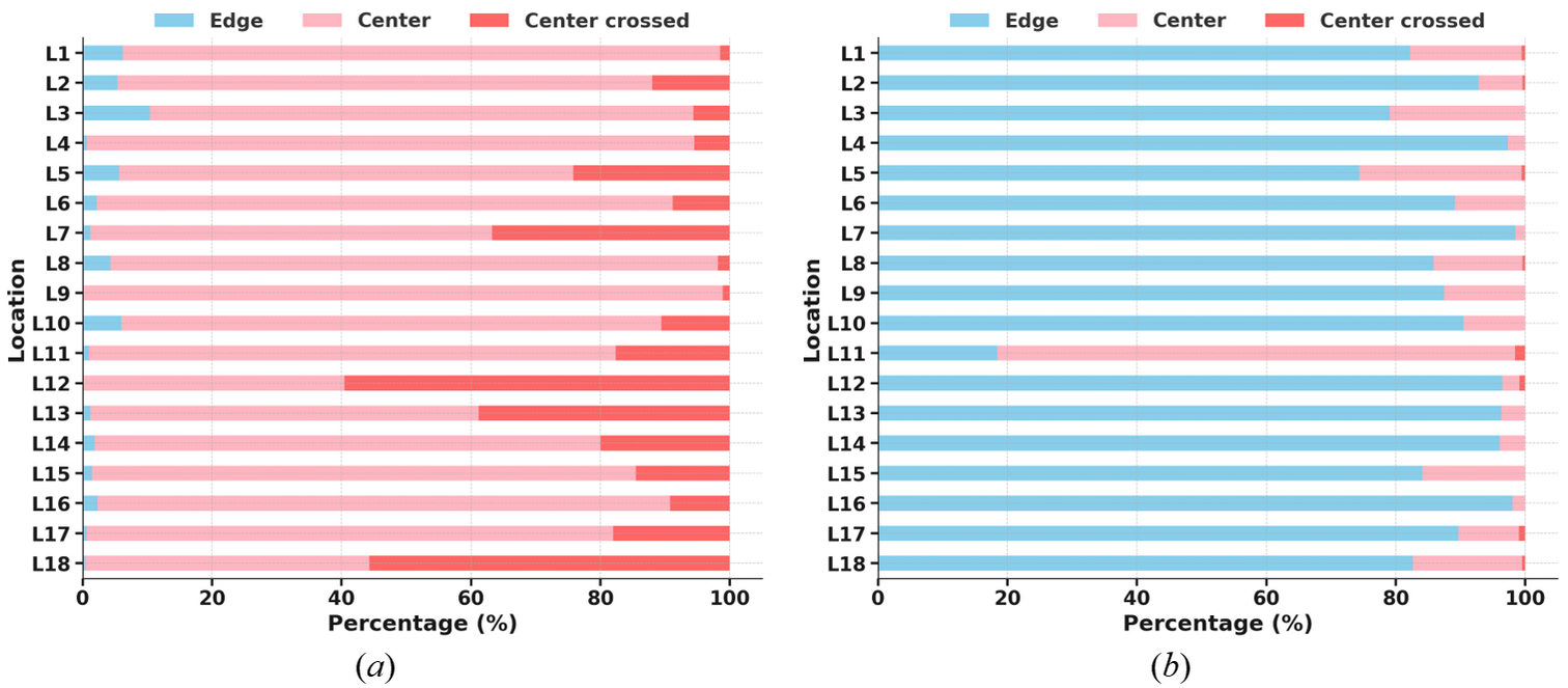
It is evident from Figure 9 that vehicles in the outer lane show a higher tendency to shift toward the centerline (pink and red), while vehicles in the inner lane predominantly shift toward the edge (blue). This suggests that outer lane vehicles are more prone to lane encroachment as compared to those in the inner lane. Further, the descriptive statistics of the proportion of lateral shifts are presented in Table 4.
| Lane | Lateral shift | Mean | Min | Max |
|---|---|---|---|---|
| Outer | Edge | 2.80 | 0 | 10.39 |
| Center | 78.24 | 40.48 | 98.90 | |
| Center crossed | 18.95 | 1.10 | 59.52 | |
| Inner | Edge | 85.51 | 18.46 | 98.52 |
| Center | 14.17 | 1.48 | 80.00 | |
| Center crossed | 0.32 | 0 | 1.54 |
However, the insights derived from the graphical representations necessitate statistical verification to determine whether the observed differences in the lateral shifting patterns between the two lanes are statistically significant. Firstly, the Chi-squared test was used to compare the proportions of vehicles shifting towards the edge, center, and center-crossed between two lanes. Secondly, the t-test was performed to examine the significance of lane-wise differences in the mean percentages of vehicles shifting towards the edge, center, and center-crossed separately. The results of these statistical tests are provided in Table 5.
| Test | Hypotheses | p-value | Remark |
|---|---|---|---|
| Chi-Squared test | Null Hypothesis (H₀): There is no significant association between lane type (inner vs. outer) and lateral shifting behavior (Edge, Center, Center Crossed) Alternative Hypothesis (H₁): There is a significant association between lane type and lateral shifting behavior |
< 0.001 | H0: not accepted |
| t-test (Edge) | Null Hypothesis (H₀): The proportion of vehicles shifting towards the edge/center/center crossed is the same in both the inner and outer lanes Alternative Hypothesis (H₁): The proportion of vehicles shifting towards the edge/center/center crossed differs between the inner and outer lanes |
< 0.001 | H0: not accepted |
| t-test (Center) | < 0.001 | ||
| t-test (Center Crossed) | < 0.001 |
Since the p-values for all tests conducted are less than 0.001, the null hypothesis (H₀) is rejected in each case. This establishes that there are significant differences in the lateral shifting behaviors of vehicles between the inner and outer lanes. Similarly, the Chi-squared test indicated that the distribution of vehicles shifting towards the edge, center, and center-crossed varies significantly with the subject lane type. Vehicles in the inner lane are more likely to shift towards the edge, while vehicles in the outer lane are more likely to shift towards the center. Further, significantly more vehicles in the outer lane cross the centerline, indicating a potential risk of lane encroachment.
4. Modeling results
4.1 Model parameters
Hyperparameter tuning is a crucial step in training machine learning models, as it enhances generalization, mitigates overfitting, and optimizes model complexity. For the LightGBM model, several hyperparameters, as listed in Table 6, require careful adjustment. Increasing n_estimators generally improves predictive accuracy, while parameters such as max_depth, subsample, subsample_freq, and colsample_bytree help regulate overfitting. A lower learning_rate can enhance model performance by refining gradient updates. reg_alpha and reg_lambda correspond to L1 and L2 regularization terms, respectively, improving model robustness and reducing overfitting. The num_leaves parameter determines model complexity while increasing min_split_gain further restricts overfitting. In this study, hyperparameter tuning was conducted on the training set to identify the optimal configuration for the LightGBM model. RandomizedSearchCV was utilized in Python for hyperparameter tuning, where it randomly selects combinations from a predefined search space instead of evaluating all possible options, making it more computationally efficient than GridSearchCV. Model performance was assessed using 3-fold cross-validation, and the best hyperparameters were selected based on the ROC-AUC score. The final optimized hyperparameters are presented in Table 6.
| Parameter | Description | Optimal values |
|---|---|---|
| n_estimators | Specifies the total number of boosting iterations | 500 |
| max_depth | Defines the maximum number of splits for base learners | 7 |
| subsample | Represents the fraction of training data randomly selected for training | 0.8 |
| subsample_freq | Determines the frequency of bagging, influencing resampling during training | 5 |
| learning_rate | Controls the step size for updating model weights in each iteration | 0.01 |
| colsample_bytree | Sets the fraction of features used for column subsampling | 0.8 |
| reg_alpha | Applies L1 regularization to reduce model complexity and prevent overfitting | 0.1 |
| reg_lambda | Implements L2 regularization to penalize large weights and enhance generalization | 0.1 |
| num_leaves | Specifies the maximum number of leaves in a single tree for base learners | 31 |
| min_split_gain | Defines the minimum loss reduction required to allow a node split | 0.01 |
4.2 Model evaluation
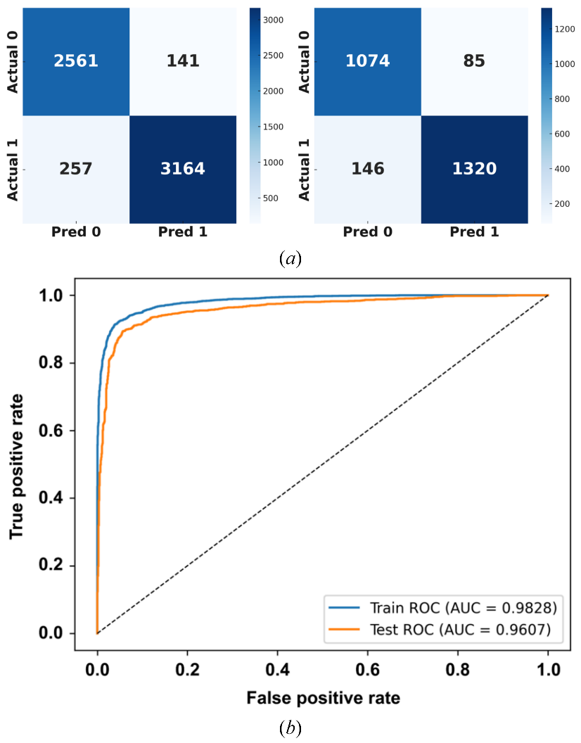
In the modeling phase, given that the LS data is a binary variable with outcomes either shifting towards the edge or towards the center, multiple evaluation metrics were employed to assess the predictive performance of the developed models. The selected metrics include Precision, Recall, Specificity, F1-score, Log-loss, AUC-ROC, and Matthews Correlation Coefficient (MCC). These evaluation metrics were chosen because predicting whether a vehicle shifts toward the centerline or edge on curved roads is a crucial safety aspect. Precision is important here because false positives, predicting a center shift when the vehicle is actually moving toward the edge, can lead to unnecessary safety interventions or misallocation of resources (Hicks et al., 2022). Recall is equally essential, as the inability to predict the true centerline shifts may fail to flag potentially risky maneuvers that increase head-on crash risks (Hicks et al., 2022). Specificity helps ensure that vehicles correctly identified as shifting toward the edge are not mistakenly treated as centerward shift (Hicks et al., 2022). The F1-score is included to assess how well the model balances these opposing needs, especially since neither error type can be ignored (Hicks et al., 2022). Log-loss adds value by evaluating the confidence of probabilistic predictions, which is vital when safety thresholds may vary across locations (Owusu-Adjei et al., 2023). AUC-ROC is chosen to assess the model’s ability to distinguish center shifts from edge shifts across all thresholds (Li, 2024). Finally, MCC is used because it reflects overall reliability and is well-suited to a balanced dataset (Hicks et al., 2022). The values from the Confusion Matrix, viz., the number of true positives (TP), true negatives (TN), false positives (FP), and false negatives (FN), were utilized to calculate the performance metrics given in Equations (7–12).
\begin{equation} \mbox{Precision} = \frac{TP}{TP + FP}\tag{7} \end{equation}A higher precision indicates fewer false positive cases.
\begin{equation} \mbox{Recall (Sensitivity)} = \frac{TP}{TP + FN}\tag{8} \end{equation}A higher recall means the model successfully identifies most of the positive instances, reducing false negatives.
\begin{equation} \mbox{Specificity} = \frac{TN}{TN + FP}\tag{9} \end{equation}A high specificity ensures fewer false positives.
\begin{equation} F1 - score = 2 \times \frac{Precision \times Recall}{Precision + Recall}\tag{10} \end{equation}A high F1-score signifies a strong balance between precision and recall.
\begin{eqnarray} Log - loss &=& - \frac{1}{N}\sum_{i = 1}^{N}\lbrack y_{i}\log\left( \widehat{y_{i}} \right)\nonumber\\ &&+ (1 - y_{i})\log(1 - \widehat{y_{i}})\rbrack\tag{11} \end{eqnarray}where yi = actual class label (yi ∈ {0,1}); \(y\widehat{i}\) = predicted probability of the positive class (P(yi = 1)); N = total number of samples. A lower log-loss value indicates better model calibration and improved probabilistic confidence.
\begin{equation} \begin{array}{l} \mbox{Matthews Correlation Coefficient (MCC)} \\ = \dfrac{(TP \times TN) - (FP \times FN)}{\sqrt{(TP + FP)(TP + FN)(TN + FP)(TN + FN)}}\tag{12} \end{array} \end{equation}It ranges from -1 to 1, where 1 indicates perfect classification, 0 means no better than random guessing, and −1 represents completely incorrect predictions.
Finally, AUC-ROC measures the area under the Receiver Operating Characteristic (ROC) curve, which evaluates the model’s ability to distinguish between positive and negative classes. A higher value indicates better differentiation between classes.
The performance of the developed model was evaluated against several widely adopted machine learning techniques. The results presented in Table 7 demonstrate that LightGBM consistently achieved superior performance in both the training and testing phases compared to other models, including AdaBoost, Random Forest, Support Vector Machine (SVM), and XGBoost. Furthermore, an analysis of training and testing performance revealed no evident signs of overfitting, suggesting that the 3-fold cross-validation strategy effectively ensures model generalization.
| Model | Phase | Precision | Recall | Specificity | F1-score | Log-loss | AUC-ROC | MCC |
|---|---|---|---|---|---|---|---|---|
| LightGBM | Train | 0.96 | 0.92 | 0.95 | 0.94 | 0.17 | 0.98 | 0.87 |
| AdaBoost | 0.96 | 0.91 | 0.95 | 0.93 | 0.67 | 0.96 | 0.85 | |
| Random Forest | 0.99 | 0.99 | 0.99 | 0.99 | 0.05 | 0.99 | 0.99 | |
| SVM | 0.96 | 0.88 | 0.96 | 0.92 | 0.27 | 0.93 | 0.83 | |
| XGBoost | 0.96 | 0.94 | 0.96 | 0.96 | 0.11 | 0.98 | 0.91 | |
| LightGBM | Test | 0.94 | 0.90 | 0.93 | 0.92 | 0.24 | 0.96 | 0.82 |
| AdaBoost | 0.95 | 0.89 | 0.95 | 0.92 | 0.67 | 0.95 | 0.83 | |
| Random Forest | 0.90 | 0.90 | 0.87 | 0.90 | 0.97 | 0.94 | 0.78 | |
| SVM | 0.96 | 0.87 | 0.95 | 0.91 | 0.29 | 0.92 | 0.82 | |
| XGBoost | 0.92 | 0.90 | 0.91 | 0.91 | 0.28 | 0.95 | 0.81 |
The confusion matrix and ROC curves for both the training and testing phases of the LightGBM model are visualized in Figure 10.
4.3 Model interpretation
An essential aspect of the analysis was the interpretation of modeling results and their translation into actionable insights. This section presents the application of SHAP to interpret the outcomes of the LightGBM model and quantify the contributions of individual factors. Additionally, uncertainty quantification was performed using the Shannon entropy method to assess the reliability and variability of the model’s predictions.
4.3.1 SHAP summary plot
The SHAP summary plot, as shown in Figure 11, provides valuable insights into the factors influencing lateral shifting behavior on horizontal curves. Red color dots represent higher feature values, while blue color dots represent lower feature values. On the other hand, higher SHAP values indicate a higher probability of shifting toward the center, whereas lower SHAP values indicate a higher probability of shifting toward the edge. Hence, from Figure 11, the following findings are extracted.
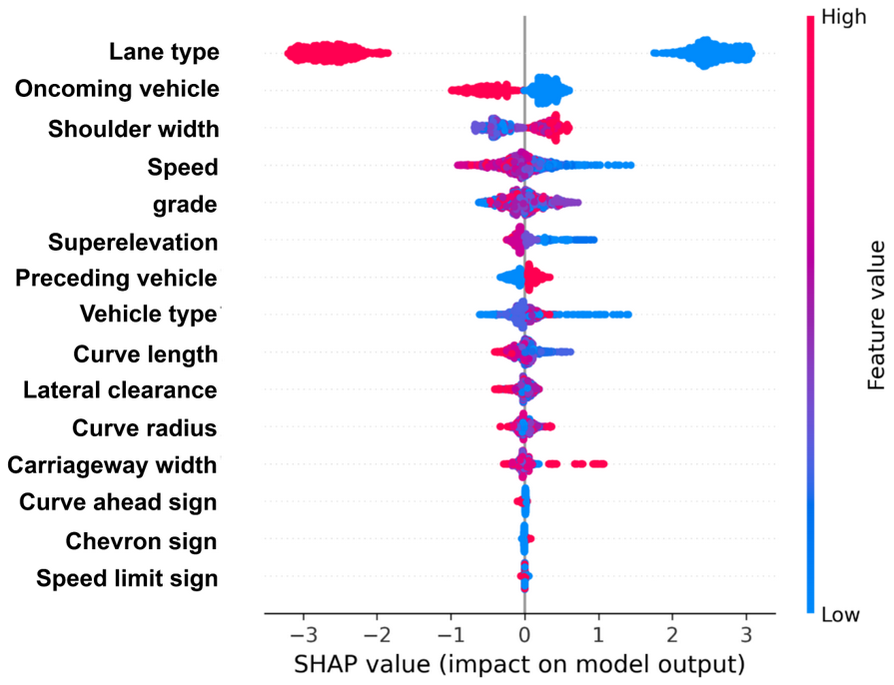
Among the most influential factors, lane type plays a crucial role in lateral shifting behavior. Vehicles in the inner lane tend to shift toward the edge line, likely to avoid head-on crashes by maintaining a safer path. In contrast, outer-lane vehicles are more inclined to shift toward the centerline, possibly taking a shorter path through the curve, reducing steering effort, and optimizing trajectory. This finding aligns with the results obtained from the Chi-square and t-test analyses conducted earlier. Similarly, vehicle speed significantly affects the lateral position of vehicles. Vehicles traveling at higher speeds have a higher probability of shifting toward the edge, while vehicles traveling at lower speeds tend to shift more toward the center. However, this general observation does not explain the variation in lateral shifting behavior with speed for vehicles traveling in the inner and outer lanes separately. Furthermore, the curve radius significantly influenced lateral shift behavior. Vehicles traversing sharp curves exhibited a tendency to shift toward the centerline, whereas those navigating gentler curves tended to shift toward the edge. This pattern can be attributed to the reduced necessity for aggressive steering corrections on gentler curves. The influence of speed and curve radius on lateral shifting for both lanes is further analyzed using the SHAP dependence plot in subsection 4.3.2.
Traffic conditions, including the presence of preceding and oncoming vehicles, significantly impact lateral shift behavior. As drivers tend to follow the preceding vehicle and shift toward the center to gain visibility. Drivers encountering oncoming vehicles exhibit a strong tendency to shift toward the edge, likely as a precaution to maintain safe lateral separation. Conversely, when no oncoming traffic is present, drivers are more comfortable maintaining a lateral position closer to the centerline of the road.
Roadway geometric characteristics and cross-sectional elements significantly influence lateral shift tendencies. A wider carriageway and shoulder width are observed to promote a shift toward the center of the road. This tendency may be attributed to the increased available space, which allows vehicles to travel closer to the center with minimal constraints. Additionally, in the presence of an oncoming vehicle, drivers can maneuver toward the edge without significant difficulty due to the ample shoulder and carriageway width. However, narrower carriageways and shoulder widths lead to shifting toward the edge due to maintaining a strict separation from the oncoming vehicles. Superelevation also plays a role in vehicle positioning, where optimum superelevation enhances lateral stability, reducing centerline encroachment and encouraging shifting toward the edge. Conversely, lower superelevation is associated with an increased likelihood of shifting toward the centerline. Similarly, longitudinal grade influences lateral positioning, with steeper slopes prompting drivers to shift toward the roadway edge due to heightened uncertainty and perceived risk. In contrast, a flatter grade is associated with more frequent shifts toward the centerline, likely due to improved driving conditions and a reduced sense of risk. Additionally, shorter curve lengths were associated with increased lateral shifting toward the centerline, possibly due to drivers' tendency to negotiate such curves more quickly with minimal steering effort.
One of the critical variables affecting visibility and driver behavior is lateral clearance, which measures the distance from inner-side obstructions to the centerline of the road. A larger lateral clearance from inner-side obstructions encourages shifting toward the edge, as increased visibility allows drivers to anticipate the curvature ahead. In contrast, a smaller lateral clearance forces drivers to move toward the center, as reduced visibility makes them uncertain about the road curvature ahead. This highlights the importance of providing adequate lateral clearance on horizontal curves to reduce unnecessary centerline encroachment and improve sight distance. A more detailed interpretation is given in subsection 4.3.2.
The influence of road infrastructural factors on lateral shifting behavior is observed to be relatively minor as compared to road geometric and traffic factors, as shown in Figure 11. However, to examine how lateral shifting behavior varies across different road infrastructural factors, a sensitivity analysis was conducted by holding all other variables constant. The results are presented in Figure 12.
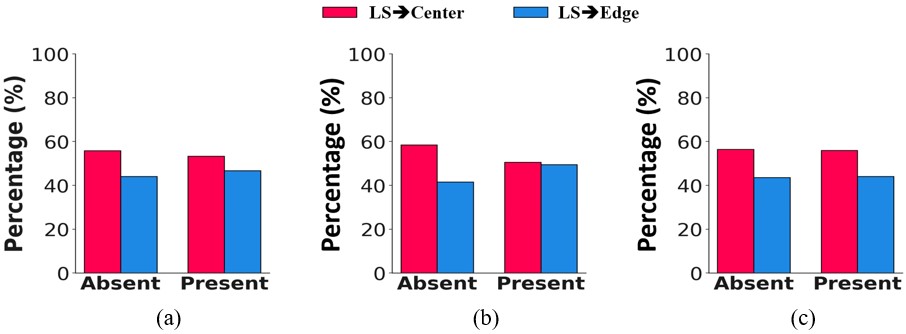
It is observed that when a speed limit sign is present, the percentage of centerline shifts decreases from 55.87% to 53.28%. A larger reduction is observed with the curve ahead sign, where lateral shift towards the centerline decreases from 58.44% to 50.54%. In the case of the chevron sign, the reduction is minimal, from 56.39% to 55.98%. These changes suggest that the curve ahead sign has the strongest influence in discouraging centerline shifting, likely because it gives drivers early warning and allows more time to adjust their position. The speed limit sign also contributes to safer lateral positioning, though its effect is moderate. The chevron sign, despite being highly visible, shows only a marginal effect. This indicates that warning-based signs, such as curve ahead, may be more effective than directional signs like chevrons in guiding lateral positioning at horizontal curves.
Further, a similar analysis was conducted for speed and the results are presented in Table 8. It reveals that the presence of Speed limit and Curve ahead signs tends to reduce vehicle speeds, with the mean speeds dropping by 6.01 km/hr and 2.22 km/hr due to the presence of Speed limit and Curve ahead signs, respectively.
| Speed (km/hr) | Speed limit | Curve ahead | Chevron | ||||||
|---|---|---|---|---|---|---|---|---|---|
| Absent | Present | Diff. | Absent | Present | Diff. | Absent | Present | Diff. | |
| Min | 15.06 | 15.02 | -0.04 | 15.02 | 15.06 | 0.04 | 15.02 | 15.09 | 0.07 |
| Max | 74.84 | 73.23 | -1.61 | 74.84 | 72.47 | -2.37 | 74.84 | 74.35 | -0.49 |
| Mean | 38.30 | 32.29 | -6.01 | 36.87 | 34.65 | -2.22 | 35.79 | 37.48 | 1.69 |
| 85th percentile | 48.86 | 45.32 | -3.54 | 48.86 | 43.50 | -5.36 | 47.12 | 50.89 | 3.77 |
This indicates that such regulatory and warning signs are effective in moderating faster-moving vehicles by alerting drivers about upcoming curve-related risks. On the contrary, the presence of Chevron signs slightly increases the mean speed by 1.69 km/hr. This suggests that chevron signs might enhance drivers’ perception of curve visibility and guidance, leading to more confident and slightly faster maneuvering. Overall, while Speed Limit and Curve Ahead signs function as cautionary controls, Chevron signs may unintentionally induce comfort-based speed increment.
A contrasting pattern of lateral shifting has been observed between inner and outer lanes as the longitudinal grade increases, as shown in Figure 13.
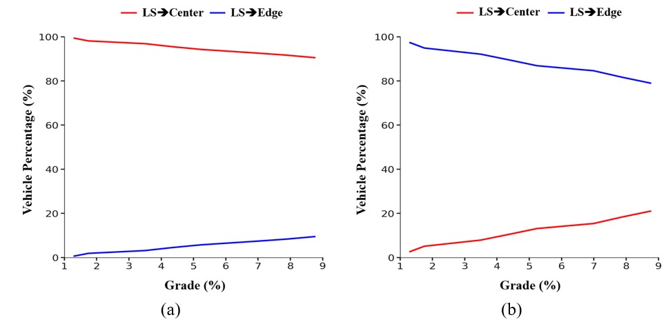
On the outer lane, the majority of vehicles consistently shift toward the center (>90%), likely to reduce curve length or steering effort. However, with increasing grade (1.31 – 8.75%), a gradual rise in edge-ward shift (from 0.64% to 9.45%) is observed. This shift may reflect increased caution due to rising uncertainty, fear of a head-on crash, and to increase the visibility at steeper gradients. Conversely, on the inner lane, most vehicles initially prefer to shift towards the edge and follow a safe path. However, as the grade steepens, the proportion of vehicles shifting toward the center increases sharply (from 2.68% to 21%), possibly to enhance visibility and perceived safety. This highlights the influence of longitudinal grade on vehicles traveling on both inner and outer lanes.
4.3.2 SHAP dependence plot
While the SHAP summary plot offers a global view of feature importance and the overall direction of their impact, it does not show how the individual factors influence predictions. This limitation is addressed by the SHAP dependence plot, which illustrates the exact relationship between a feature and its SHAP value, capturing non-linear trends and threshold effects that summary plots overlook. Additionally, it enables interaction analysis with a second feature (e.g., lane type), revealing how the effect of one variable may depend on another. This makes dependence plots especially useful for uncovering conditional patterns and hidden dependencies, thereby providing a more detailed, instance-level understanding of model behavior. Therefore, to further quantify the impact of individual factors on the LightGBM model's output, some selected SHAP dependence plots are presented in Figure 14 to demonstrate their specific effects.
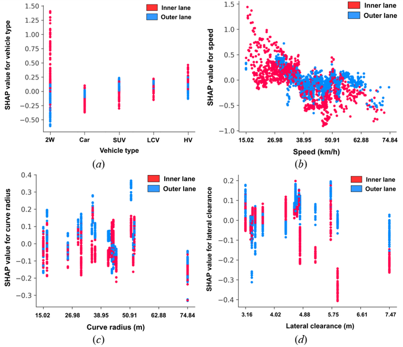
Figure 14a shows the SHAP dependence plot for vehicle type and provides key insights into how different vehicle categories influence lateral shifting behavior. The horizontal axis represents the vehicle type, ranging from 2W to HV, while the left vertical axis shows the SHAP value, indicating each vehicle type's contribution to predicting lateral shift. The right vertical axis (color bar) represents Lane Type, where blue corresponds to the outer lane and red represents the inner lane. The plot reveals that 2W exhibits the strongest tendency of lateral shift, irrespective of shifting toward the centerline or edge line, as indicated by the highest and lowest SHAP values as compared to other vehicle types. This behavior is likely due to their smaller size and greater maneuverability, allowing them to navigate closer to the center or edge without stability concerns. Among Cars, SUVs, and LCVs, vehicles traveling in the inner lane exhibit a greater tendency to shift toward the edge compared to those in the outer lane. However, as vehicle size increases, a slight shift toward the centerline is observed. On the contrary, for HVs, inner lane vehicles demonstrate a slight tendency to shift toward the center, whereas outer lane vehicles exhibit a greater inclination to shift toward the edge, but they still remain lower than those for two-wheelers.
The SHAP dependence plot for Speed (Figure 14b) reveals some unique speed-based trends in lateral shifting behavior. At very low speeds (15.02–26.98 km/h), vehicles exhibit high positive SHAP values (0.5–1.5), indicating a strong tendency, for both inner and outer lane vehicles, to move toward the center of the road. However, this behavior is more pronounced for inner lane vehicles (red dots), suggesting that lower speeds provide greater maneuverability, allowing drivers to position themselves closer to the center to increase their visibility. As speed increases into the moderate range (26.98–38.95 km/h), SHAP values gradually decrease, reflecting a transition from movement toward the center to a more ideal lateral position. While inner-lane vehicles still show some preference for the center, outer-lane vehicles (blue dots) begin shifting slightly toward the edge of the road. In a relatively higher speed range (38.95–50.91 km/h), the majority of SHAP values remain below zero, indicating a gradual lateral shift toward the edge. Inner lane vehicles exhibit a tendency to drive closer to the edge, while outer lane vehicles maintain a more controlled trajectory with a slight outward shift toward the edge. However, as speed increases beyond 50.91 km/h, inner lane vehicles exhibit a strong tendency to shift toward the edge, as indicated by SHAP values reaching as low as -0.2. This suggests that drivers traveling at high speeds actively move away from the center of the road. Inner lane vehicles demonstrate the most pronounced tendency to shift toward the edge as the speed increases, highlighting the critical influence of lane positioning on speed-induced lateral shifting behavior.
The SHAP dependence plot for Curve Radius is exhibited in Figure 14c. For sharp curves (25.02–39.19 m), SHAP values are predominantly positive for outer lane vehicles, indicating a strong tendency for vehicles to shift toward the center. This behavior is expected, as sharper curves require more significant steering adjustments, leading to overcorrection. Vehicles in the inner lane (red dots) exhibit a stronger shift toward the edge than those in the outer lane. In moderate curve radii (39.19–67.52 m), SHAP values show greater variability, with some vehicles shifting toward the center (positive SHAP values) and others shifting toward the edge (negative SHAP values). This suggests that lane positioning in moderately curved segments is influenced by additional factors such as speed, visibility, and other driver-level factors. Inner lane vehicles still display a greater tendency to shift toward the edge compared to outer lane vehicles, but the variation in SHAP values indicates a mix of behaviors across different driving conditions. For gentle curves (67.52–100 m), SHAP values trend negative, meaning vehicles on both lanes are more likely to shift toward the edge. This behavior can be attributed to the reduced steering effort required in gentle curves, which allows drivers to maintain a stable position closer to the road’s edge without significant maneuvering.
Figure 14d presents the SHAP dependence plot for Lateral clearance. For values between 3.16 and 4.45 m, SHAP values are mostly positive for the inner lane, suggesting a higher likelihood of shifting toward the centerline, probably to increase their visibility. Similarly, the SHAP values for the outer lane are mostly negative, indicating shying away from the centerline to increase their visibility as well. This indicates that when the lateral distance from inner-side obstructions is small, both inner and outer lane drivers tend to adopt a strategy to gain visibility and counter perceived spatial constraints. As this value increases from 4.55 to 7.47 m, a distinct pattern emerges. Outer lane drivers (blue dots) exhibit positive SHAP values, indicating a tendency to shift toward the centerline as lateral clearance increases. Improved visibility and perceived safety likely boost driver confidence, prompting them to follow a straighter trajectory through the curve, requiring less steering effort. Conversely, inner lane drivers (red dots) exhibit negative SHAP values, indicating a tendency to move toward the edge as lateral clearance increases. This suggests that greater lateral clearance allows inner lane drivers to stay farther from the centerline, possibly due to improved visibility of the curve ahead.
4.3.3 Uncertainty quantification
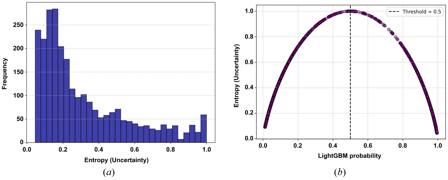
While SHAP analysis reveals which features influence a model’s prediction and explains why a certain output was generated, it does not indicate how confident the model is in that prediction. This limitation is critical in binary classification tasks, such as predicting lateral shifting behavior, where continuous probabilities are reduced to hard labels (0 or 1), potentially forcing uncertain predictions near the threshold (e.g., 0.5) into definitive decisions. To overcome this, Shannon’s entropy was employed to quantify predictive uncertainty, with entropy peaking near 0.5 (maximum uncertainty) and decreasing toward 0 or 1 (high confidence). The entropy distribution (Figure 15a) shows how often the model produces low-confidence outputs, while the entropy vs. probability plot (Figure 15b) confirms that uncertainty is highest near the threshold. This analysis offers an essential dimension that SHAP alone cannot capture, distinguishing between reliable and ambiguous predictions. Without it, one risks over-trusting decisions that appear interpretable but may be uncertain, making entropy analysis essential for ensuring both interpretability and confidence in model outputs.
The predictive entropy analysis, illustrated in Figure 15a, highlights strong model performance with minimal uncertainty in most cases. The entropy distribution indicates that the majority of predictions exhibit low uncertainty, with a mean entropy of 0.316 and a standard deviation of 0.248, suggesting the model is generally confident in its classifications. The majority of entropy values fall below 0.5, with the 25th percentile at 0.132, the median at 0.218, and the 75th percentile at 0.450, reinforcing that most predictions are well-defined. However, 144 out of 2625 predictions (5.5%) exceed the 0.85 entropy threshold, indicating high uncertainty in a small subset of cases.
The entropy vs. LightGBM probability plot, depicted in Figure 15b, further reinforces this analysis by revealing that uncertainty is highest when predicted probabilities are near 0.5, which aligns with theoretical expectations in a binary classification task. The entropy curve exhibits a distinct inverted U-shape, confirming that probabilities closer to 0 or 1 have lower entropy, indicating higher classification confidence when predicting a lateral shift toward the edge or center, respectively. This behavior is desirable as it suggests that the model can confidently predict the lateral shifting behavior for the majority of instances while acknowledging uncertainty in borderline cases.
5. Discussion
The study aimed to identify and interpret the effects of various key factors influencing the lateral shifting behavior of vehicles on hilly horizontal curves, particularly under the LMIC setting. A total of 15 key input variables, comprising eight continuous and seven categorical variables, were used to model the lateral shifting (LS) behavior. The model's performance was evaluated using multiple metrics, including Precision, Recall, Specificity, F1-score, Log-loss, AUC-ROC, and Matthews Correlation Coefficient (MCC), all of which indicated satisfactory performance (Table 7). Further comparison with other ML-based models, namely XGBoost, AdaBoost, Random Forest, and SVM, revealed that LightGBM consistently demonstrated superior overall performance. This was followed by a SHAP analysis that provided several important insights into LS behavior on hilly horizontal curves. Some of these insights are discussed below.
One of the most pronounced findings is the strong influence of lateral clearance, defined as the lateral distance from the inner-side obstruction (such as a hill or vegetation) to the centerline of the road. Inner lane vehicles showed a clear tendency to shift toward the centerline when lateral clearance was low. This behavior is likely due to their closer proximity to the obstruction, prompting drivers to move away to improve their visibility of the road ahead. A similar observation was reported by Bassani et al. (2019) for inner lane vehicles. However, the present study also found that outer lane vehicles displayed a comparable compensatory response by shifting outward toward the edge to enhance visibility when lateral clearance was low. This contrasts with Bassani et al. (2019), who reported that outer lane vehicles, being farther from the obstruction and enjoying inherently better visibility and a greater sense of safety, did not exhibit such adjustments and laterally shifted towards the center. Finally, the SHAP analysis revealed a lateral clearance threshold (~4.5 m), below which drivers shift away from obstructions to enhance visibility, but beyond which further clearance has little impact on lateral shifting behavior.
Further, the SHAP dependence plot revealed various interesting insights between speed and the lateral shifting behavior. At lower speeds, inner lane vehicles tend to shift toward the centerline. This represents a compensatory action by drivers to increase curve visibility, while maintaining a low speed during this maneuver reflects a strategic effort to avoid possible crashes, an aspect previously unexplored.
A similar strategic action was observed among outer lane vehicles at lower speeds, wherein they tended to shift toward the centerline and even encroached on it to follow a straighter trajectory through the curve, thereby minimizing steering effort. This maneuver, however, was executed at lower speeds, likely to retain sufficient control and allow evasive action if an oncoming vehicle appeared, thus reducing head-on crash risk. In contrast, Fitzsimmons et al. (2013) reported that at lower speeds, outer lane vehicles were more likely to shift toward the edge, favoring a more stable and cautious trajectory. At higher speeds, inner lane vehicles were observed to shift toward the edge, possibly to avoid encroaching into the opposing lane. This pattern differs from the findings of Fitzsimmons et al. (2013), who observed that inner lane vehicles tended to shift toward the centerline at higher speeds. Similarly, outer lane vehicles in the present study were observed to drift toward the edge, possibly due to the influence of higher centripetal forces. In contrast, Fitzsimmons et al. (2013) reported that outer lane vehicles tend to shift toward the centerline, engaging in a cutting maneuver. This clearly indicates that a strong relationship exists between vehicle speed and the driver's perception of curve safety and visibility, with speed likely influenced by how safe and visible the curve appears to the driver.
Additionally, the present study observed the influence of diverse vehicle types on the lateral shifting behavior. The SHAP dependence plot revealed that two-wheelers (2W) exhibited the strongest tendency to shift toward the centerline when traveling on the inner lane and toward the edgeline when on the outer lane, likely due to their higher maneuverability compared to larger vehicles. Fitzsimmons et al. (2013) reported a similar tendency in 2W but observed only centerline-cutting behavior. Similarly, the present study found that, after two-wheelers (2W), heavy vehicles (HV) also exhibited a comparable shifting pattern. In contrast, Fitzsimmons et al. (2013) reported that HV generally maintained a more stable path. However, cars, SUVs, and LCVs exhibited a lateral shifting tendency opposite to that of two-wheelers and heavy vehicles, consistent with the findings of Fitzsimmons et al. (2013). This shows that two extreme vehicle types, 2Ws and HVs, exhibit similar shifting patterns. In contrast, Cars, SUVs, and LCVs follow an opposite but consistent pattern, indicating that vehicle size and weight are not the sole factors influencing lateral positioning at curves.
The study also examined the influence of oncoming and preceding vehicles. In the presence of oncoming vehicles, drivers tended to shift toward the edge, likely to increase the lateral buffer and reduce perceived collision risk. In contrast, when a preceding vehicle was present, drivers often aligned their lateral position with it or shifted slightly toward the centerline, suggesting that such adjustments are driven more by visibility needs than safety concerns.
Table 9 presents a comparison of the current findings with those of existing studies, emphasizing both consistencies and contradictions in observed lateral shifting behavior.
| Influencing factors | Positive relationship | Negative relationship |
|---|---|---|
| 1. Lane type | ||
| a) Outer lane | This study; Fitzsimmons et al. (2013) | |
| b) Inner lane | This study | |
| 2. Speed | (Fitzsimmons et al., 2013; Hallmark, 2012; Stodart et al., 2008) | This study |
| 3. Oncoming vehicle | This study | |
| 4. Preceding vehicle | This study | |
| 5. Curve radius | This study; (Bassani et al., 2019; Ben-Bassat & Shinar, 2011; Charlton, 2007; Das et al., 2016; Glennon & Weaver, 1971; Maljković & Cvitanić, 2016; Mauriello et al., 2018; Stodart et al., 2008) | |
| 6. Curve length | This study | |
| 7. Lateral clearance | This study (for outer lane vehicles) | This study (for inner lane vehicles); Bassani et al. (2019) (for both inner and outer lane vehicles) |
| 8. Carriageway width | This study; Das et al. (2016) | |
| 9. Shoulder width | This study | |
| 10. Superelevation | This study (at optimum superelevation); Glennon & Weaver (1971) | |
| 11. Grade | This study; Stodart et al. (2008) (When avg. grade ≥ |5%|) | |
| 12. Speed limit sign | This study | |
| 13. Chevron sign | This study; Charlton (2007) | |
| 14. Curve ahead sign | This study | |
| 15. Vehicle types | ||
| a) 2W | This study (when traveling on the inner lane); Fitzsimmons et al. (2013) | This study (when traveling on the outer lane) |
| b) Car, SUV, and LCV | This study (when traveling on the outer lane); Fitzsimmons et al. (2013); | This study (when traveling on the inner lane) |
| c) HV | This study (when traveling on the inner lane; Das et al. (2016) | This study (when traveling on the outer lane) |
6. Conclusion
The present study employed LightGBM to model vehicle lateral shifting behavior on two-lane undivided hilly horizontal curves, considering a range of road geometric, traffic, and infrastructural factors. LightGBM was chosen over traditional regression models, commonly used in previous studies due to its superiority in capturing complex, non-linear interactions among multiple variables. To address the model’s black-box nature, SHAP-based interpretation was used to enhance transparency and identify key influencing factors. Both SHAP summary and dependence plots were adopted, the former to rank overall feature importance, and the latter to explore how individual factors and their interactions influence the model output. The analysis offered new insights into the role of less-explored factors such as curve length, longitudinal grade, lateral clearance, the presence of oncoming or preceding vehicles, curve ahead signage, and a wide range of vehicle types (2W, Car, SUV, LCV, HV).
6.1 Key insights
-
On comparing five popular ML-based approaches, the LightGBM-based LS model was observed to perform best overall, with consistent results in both the training and testing phases.
-
Lateral clearance was found to be one of the primary contributors to lateral shift at a horizontal curve. Below 4.5 m of lateral clearance on the inner side of the curve, drivers compensate for poor visibility: inner-lane vehicles drift toward the center and outer-lane vehicles shift toward the outer edge. Beyond this threshold, the lateral clearance has an insignificant influence on the lateral shift of vehicles.
-
At low speed (< 27 km/h), vehicles on both lanes tend to shift towards the center for better visibility. While with rising speed (> 39 km/h), the vehicle laterally shifts toward the edge.
-
Vehicles tend to shift towards the center at sharp curves (curve radius < 39 m), while gentler curves result in better lane keeping.
-
Oncoming vehicles were observed to induce lateral shift toward the edge, while the presence of a preceding vehicle draws them slightly toward the center for better visibility.
-
On the outer lane, the percentage of edgeward shift increases from 0.64% to 9.45% as longitudinal grade rises from 1.31% to 8.75%. While on the inner lane, centerward shifts rise from 2.68% to 21% over the same grade range, indicating visibility-seeking and risk-avoidance across both lanes.
-
Among five vehicle classes, two-wheelers and heavy vehicles exhibit the most pronounced bi-directional pattern, with inner lane vehicles shifting toward the center and outer lane vehicles shifting toward the edge. Whereas Cars, SUVs, and LCVs show an opposite pattern, indicating that maneuverability and driver strategy also govern the lateral positioning behavior of vehicles rather than vehicle size alone.
-
The curve-ahead sign yields the largest reduction in centerward shifts (8.0%). The speed-limit sign has a moderate effect (2.6%) on the lateral shift, while the chevron sign does not have a significant impact. However, the speed-limit sign was the most effective for speed control, lowering the mean speed by 6 km/h.
6.2 Policy implications and limitations
-
A minimum lateral clearance of 4.5 m needs to be ensured on the inner side of a horizontal curve on a hilly highway. This can be done by regular vegetation trimming and targeted removal of roadside rocks or soil cutbacks within 4.5 m of the inner edge of the road.
-
Maintaining proper lateral position and encouraging driving near the edge can be encouraged on sharp curves by adding edge guidance. This can be done by using bold edge lines. Further, centerline cutting may be discouraged by providing centerline buffers or double center lines.
-
After each intervention, centerline encroachments can be monitored by lane type and speed interval and next steps can be decided accordingly.
-
Vehicle classes with high variability in lateral shifting behavior, such as two-wheelers and heavy vehicles, can be targeted with supportive measures. Local awareness programs can be conducted to improve the awareness about the lateral shifting issues and other safety concerns related to driving at undivided two-lane horizontal curves among the drivers of two-wheelers and heavy vehicles, particularly in hilly regions.
However, this study is not without limitations. First, while a high-mounted video recorder was used to capture vehicle movements with reasonable accuracy, future studies may adopt more advanced methods, such as drone-based video recording, to achieve higher precision. Secondly, the effects of adverse weather and low-visibility conditions (e.g., rain or fog) were not considered, presenting an opportunity for future research to explore driver behavior under such environmental challenges.
CRediT contribution statement
Samrat Debbarma: Conceptualization, Data curation, Formal analysis, Investigation, Methodology, Software, Visualization, Writing—original draft, Writing—review & editing. Wahengbam Ratankumar: Data curation, Software, Writing—original draft. Subhadip Biswas: Conceptualization, Formal analysis, Methodology, Supervision, Validation, Writing—review & editing.
Declaration of competing interests
The authors report no competing interests.
Declaration of generative AI use in writing
During the preparation of this work, the authors used GPT-4 to check writing for grammatical errors and improve clarity of language in the final manuscript. The outputs were reviewed and revised by the authors, who take full responsibility for the content of the publication.
Ethics statement
The research conducted in this study does not involve human subjects and is therefore exempt from ethical review or approval.
Funding
No external funding was used in this research.
Editorial information
Handling editor: Carmelo D'Agostino, Lund University, Sweden.
Reviewers: Bhadradri Raghuram Kadali, National Institute of Technology Warangal, India; Hari Krishna Gaddam, Gati Shakti Vishwavidyalaya, India.
Submitted: 27 March 2025; Accepted: 6 December 2025; Published: 19 December 2025.