Extreme Value Analysis for Safety Benefit Estimation of Adaptive Cruise Control (ACC)
Abstract
As new automated features enter the automotive market, we need methods to assess their safety in a rapid, proactive, and iterative way. The traditional way of relying on crash statistics does not meet these needs. An alternative is to use extrapolation techniques designed to deal with rare events, such as extreme value theory (EVT). In this paper, we applied EVT to estimate the risk of collision with and without adaptive cruise control (ACC) during steady-state car following. We defined a Bayesian regression model to estimate the parameters of the Weibull distribution for block maxima (BM) of the brake threat number (BTN). We used a small, open-access dataset collected during a platooning experiment on a test track, with and without ACC. We found that it is extremely unlikely that the use of ACC will result in a rear-end crash under normal car-following circumstances, a finding consistent with the general expectation that ACC is safer than manual driving. However, we found that the relative risk of ACC was actually higher than the human control baseline. The reason is that the baseline represents a cautious driving style which may not be typical of the driving style in real traffic. Nonetheless, EVT can measure the expected safety benefit of a vehicle system even without a large dataset. The BTN was an appropriate safety metric to compare automated and manual driving modes, as it accounts for specific brake behavior and performance.
1. Introduction
Adaptive cruise control (ACC) is a common advanced driver assistance system (ADAS) that increases comfort by reducing the effort of continuous longitudinal control. ACC can also reduce the exposure to critical lead-vehicle situations (e.g., rear-end crashes) by keeping a fixed headway to the vehicle in front. Without ACC, drivers may often tailgate so that they would not have enough time to evade a conflict (General Motors Corporation Research and Development Center, 2005, Ch. 8; Malta et al., 2012, Ch. 4). ACC is considered safer than manual control because it reduces the frequency of short (less than 1 s) headways (General Motors Corporation Research and Development Center, 2005, Ch. 8; Malta et al., 2012, Ch. 4), but the collision risk has not been quantified.
It is still unclear how to measure the real-world safety benefits of systems like ACC directly. Traditionally, safety benefit analyses have relied on crash statistics to estimate safety without automation (e.g., Otte et al., 2003). However, crashes are rare and highly varied, because they are the result of specific driver-vehicle-system dependencies (Coughlin et al., 2011), various failure mechanisms (Singh, 2015), and the co-occurrence of unexpected events (Victor et al., 2015), so it would take too long to collect a representative sample and design timely countermeasures. Safety assessments of automated systems have mainly focused on autonomous emergency interventions (e.g., autonomous emergency braking [AEB]) rather than on sustained automation (e.g., convenience systems like ACC). In fact, current crash databases may be insufficient to investigate the effects of current (and newer) ADASs, because not only is the market penetration of these systems still low, but their operation during a crash is not reported (Otte et al., 2003).
As more consumer vehicles are equipped with ADASs (and more sophisticated forms of automation), we need a method to rapidly and proactively evaluate the vehicles’ safety, based on the systems’ technological risks and benefits (Blumenthal et al., 2020), and improve them accordingly (Åsljung et al., 2017). Of the multiple alternatives to using crash data, the most common is to use near-crashes (or other crash surrogates) derived from naturalistic driving data (e.g., Dingus et al., 2006) in combination with simulations (e.g., Kusano & Victor, 2022; Olleja et al., 2022). Near-crashes are convenient as they are more frequent than crashes, but their generalizability is debated (Dozza, 2020; Tarko, 2012). We used Extreme Value Theory (EVT; Coles, 2001), which extrapolates extreme, rare events (crashes) from a set of observations of the process under study (normal driving). This approach does not require the direct observation of conflicts, as it relies on normal driving data. Further, EVT requires much shorter observation periods than other methods, so it could quantify the safety benefit of ADASs as they are deployed, accelerating their development.
Multiple studies have applied EVT to estimate the collision risk under human control (e.g., Åsljung et al., 2017; Farah & Azevedo, 2017; Orsini et al., 2020, 2021; Songchitruksa & Tarko, 2006; Tarko, 2012); a few have investigated highly automated driving (e.g., Kamel et al., 2022). In this paper, we compare rear-end crash frequency in vehicles under human control to those using ACC. Rear-end crashes are the most common type of conflict, and ACC is the most common automated feature installed in consumer vehicles that could prevent them.
2. Methods
2.1. Data source
Data come from OpenACC (Anesiadou et al., 2020; Makridis et al., 2020), an open-access dataset created to benchmark ACC during normal operation in high-end consumer vehicles. The data were collected over multiple test-track and open-road tests. Metrics such as speed, acceleration, and headway were recorded from the CAN bus and additional sensors. The dataset was sampled at 10 Hz.
We selected the data from the test-track experiment at AstaZero in Sweden, because it was the only experiment in OpenACC that included a human control baseline, which was necessary to assess the relative safety benefit of driving with automation. The experiment consisted of a platoon of five vehicles on a traffic-free rural road. The first vehicle in the platoon occasionally perturbed the other vehicles by setting a different ACC target speed. Across trials, the following vehicles remained the same, but changed their relative order in the platoon. There was no other traffic on the test-track. The participants were professional drivers.
In all trials but one, the ACC’s time headway was set at the lowest (about 1.2 s); for consistency, we discarded the single trial that had the ACC headway set to high (above 2 s). While the headway setting may seem aggressive, users generally prefer a short time gap to reduce cut-ins (General Motors Corporation Research and Development Center, 2005, Ch. 4). We also kept only those driving segments where the minimum speed of the whole platoon was more than 30 km/h (the typical minimum operating speed of ACC) for at least 10 s, in order to assess steady-state (under regime) driving. Finally, the platoon was broken down into independent pairs of vehicles (e.g., the second and third vehicles in the platoon became the leader and follower vehicle, respectively) because we were interested in understanding rear-end crash scenarios rather than the effects on the whole platoon. We assumed that drivers would not anticipate the lead-vehicle actions by looking further ahead in the platoon. Additionally, we did not study ripple (string) effects from the behavior of the following vehicle to the vehicles behind. Overall, the amount of data we retained corresponded to approximately 888 km.
2.2. Threat measure
We used the brake threat number (BTN; Brännström et al., 2008) as a surrogate measure for lead-vehicle conflicts. BTN quantifies the brake effort needed to avoid a collision by comparing the minimum acceleration (maximum deceleration) required to avoid a collision and the minimum acceleration that the brake system is capable of :
with BTN in the domain. When BTN is greater than 1, the collision cannot be avoided as the required brake effort exceeds the brake capacity. Because BTN depends on braking behavior and performance, it is an improvement over the classic time to collision (TTC) measure (Åsljung et al., 2016).
We used a simplified brake profile. First, braking is applied after a delay (Figure 1). Then, the acceleration decreases linearly with rate The braking capacity saturates when it reaches (Brännström et al., 2008). The specific ACC implementations and brake system characteristics of the vehicles in OpenACC are not publicly available. Therefore, we used reference values from current regulations or previous studies (Table 1). We did not include an AEB system to focus solely on the effect of ACC.

| Parameter | Driving mode | Value | Reference |
|---|---|---|---|
| Manual | 1.15 s | [@457238 p. 30] | |
| ACC | 0.1 s | [@457241 p. 104] | |
| Manual | -12.9 | [@457238 p. 30] | |
| ACC | -12.9 | [@457238 p. 30] | |
| Manual | -7.74 | [@457238 p. 30] | |
| ACC | -7.74 | [@457238 p. 30] |
We computed BTN in the scenario where the lead vehicle maintains its current acceleration while the vehicle behind adapts its acceleration to avoid a collision (Figure 1). The BTN has a closed-form solution in some specific cases (Åsljung et al., 2017; Brännström et al., 2008). Here, we computed it as the solution to an optimization problem instead. This approach is more computationally demanding but more flexible, as it allows both vehicles to have any (continuous or piecewise) brake profile (see Appendix). We computed the BTN for all vehicles in the platoon at every second, given the current kinematic state of the vehicles from the data (a 1 Hz frequency was chosen to reduce computational cost). The time horizon was set to 30 s, to accommodate non-critical events. All BTN values less than or equal to zero indicate that the situation did not require braking and thus were excluded.
2.3. Extreme values analysis
The values for BTN were analyzed with EVT to estimate the probability of a rear-end crash. The premise is that car-following is a set of circumstances that has a non-zero probability of ending up in a conflict, so that when the process is repeated enough times it will result in a crash. The assumption is that car following is a stationary process (Coles, 2001, Ch. 1). Crashes that are the result of exceptional lead-vehicle situations (e.g., a lead vehicle slamming on the brakes suddenly) are not considered in this analysis, as these situations would violate that assumption; the stability of the prevailing car-following process would be disrupted, and the situation would not be compatible with an EVT analysis.
2.3.1. Block maxima
We chunked the BTN time series into 7 km-long blocks. This block length was chosen to minimize temporal dependency (Coles, 2001, Ch. 5) and retain the most data (Figure 2). Then, we extracted the maximum BTN value in each block (block maxima [BM]). On average, trials were about 21 km long, resulting in about 3 BM for each vehicle in each trial. Blocks shorter than 75% of the desired block length (which can occur at the very end of the trial) were discarded.

2.3.2. Statistical model
The BM were grouped by driving mode (ACC vs. human control). Typically, the probability distribution of BM is inferred with the Generalized Extreme Values (GEV) distribution, which unites the reverse Weibull, Gumbel, and Fréchet families (Coles, 2001, Ch. 3). Given the known boundary conditions of BTN in the domain we opted for the positively defined Weibull distribution, instead of fitting the more general, yet more complex, GEV distribution. While the Fréchet distribution (a GEV component that is lower-bounded) was considered, its characteristic long right tail does not accurately represent our data. Overall, the Weibull distribution was more suitable for our analysis, although it somewhat deviates from traditional EVT applications. The Weibull distribution has two parameters (scale and shape Bürkner, 2022) and the formula
To estimate when a crash will occur, we estimated the probability that the critical value for BTN would be exceeded in the block To do so, we inferred the parameters of the Weibull distribution that best mimicked the observations (Coles, 2001, Ch. 3). The inference was performed for each driving mode using a Bayesian regression model (Bürkner, 2021):
The regression was set up to infer the mean (expected value) of the Weibull distribution instead of the scale parameter directly. The factor was the driver {0: Human; 1: ACC} associated with each data point, We used the index-variable approach to assign a unique intercept to each parameter for the specific driving mode, so we could assign priors to each mode independently (McElreath, 2019, Ch. 5). We set vague (but regularizing) priors to prevent divergences
The data were analyzed using R (v. 4.2.1; R Core Team, 2022) and the package brms (v. 2.18.0; Bürkner, 2016). We sampled 25 Markov Chain Monte Carlo (MCMC) chains with the No-U-Turn-Sampler (NUTS; Hoffman & Gelman, 2014), with 10k samples each; 5k were used as warm-up and then discarded, resulting in a total of 125k samples available for analysis. The MCMC chains (i.e., posterior distributions) carried all the information used for statistical inference.
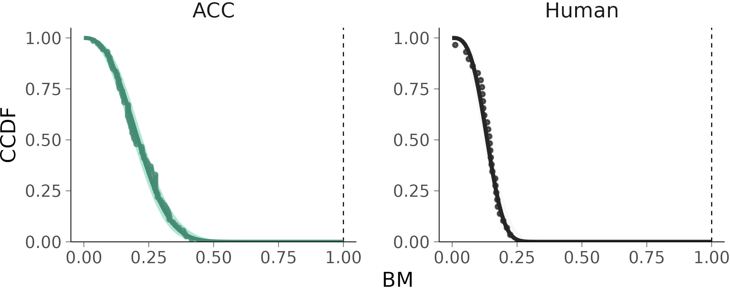
The goodness of fit for each model was assessed by comparing the posterior predictive distribution against the empirical data (posterior predictive check; Gabry et al., 2017). We used three types of plots to inspect the outcome of the statistical modeling. The first plot compared the modeled Weibull’s PDF with the normalized histogram of the data. The second plot compared the complementary cumulative distribution function (CCDF) to the complementary empirical CDF of the data Given an ordered sample of BM, the is (Coles, 2001, pp. 208, 36)
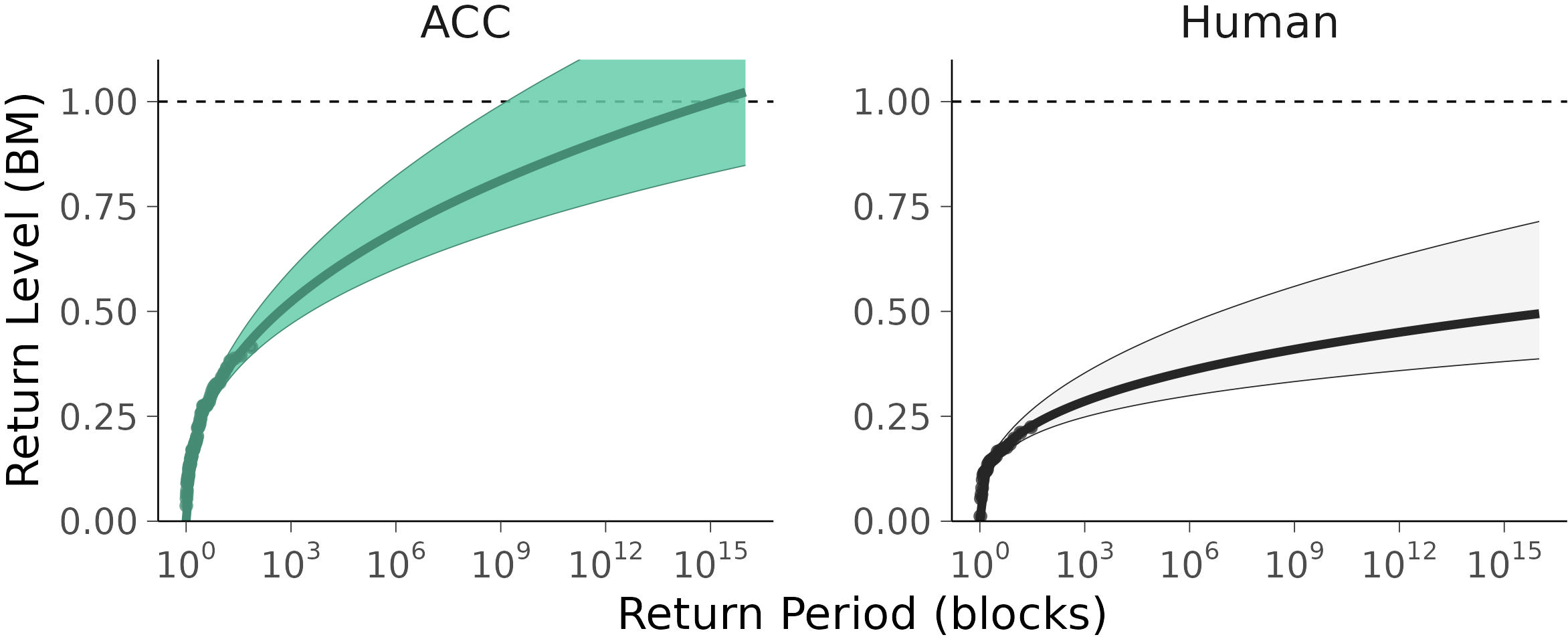
The third plot was the return plot (Coles, 2001, Ch. 3). The return plot can be used to check the model against the empirical observations, and it is also the traditional way of interpreting the outcome of an EVT analysis. The return plot shows the return levels (RLs) against return periods (RPs), often in the log scale. That is, it shows the value that is likely to be exceeded, on average, once in that RP (Coles, 2001, Ch. 3). The empirical is the observed while the empirical is calculated as
The estimate for the was computed from the regression model for a range of (typically a logarithmic series), via the inverse CDF of the Weibull distribution:
where can be interpreted as the probability of the event occurring in any given block. In other words, the probability that an event will exceed a certain threshold in any given block means that, on average, the event will occur once every blocks. In summary, for the empirical returns, we calculated the associated with a specific while for the modeled returns, we calculated the associated with a specific
The statistics for the posterior distribution were derived from manipulating the samples in the MCMC chains with the support of the packages tidybayes (v. 3.0.7; Kay, 2024) and tidyverse (v. 2.0.0; Wickham et al., 2019). For convenience, the probability distribution of a parameter/metric was summarized by the median and the 89% percentile interval (PI; McElreath, 2019, Ch. 3).
3. Results
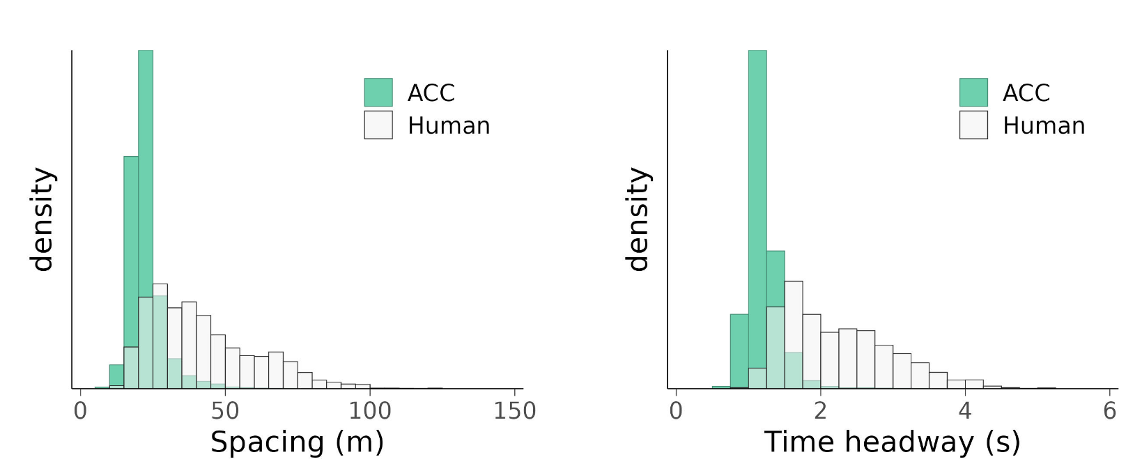
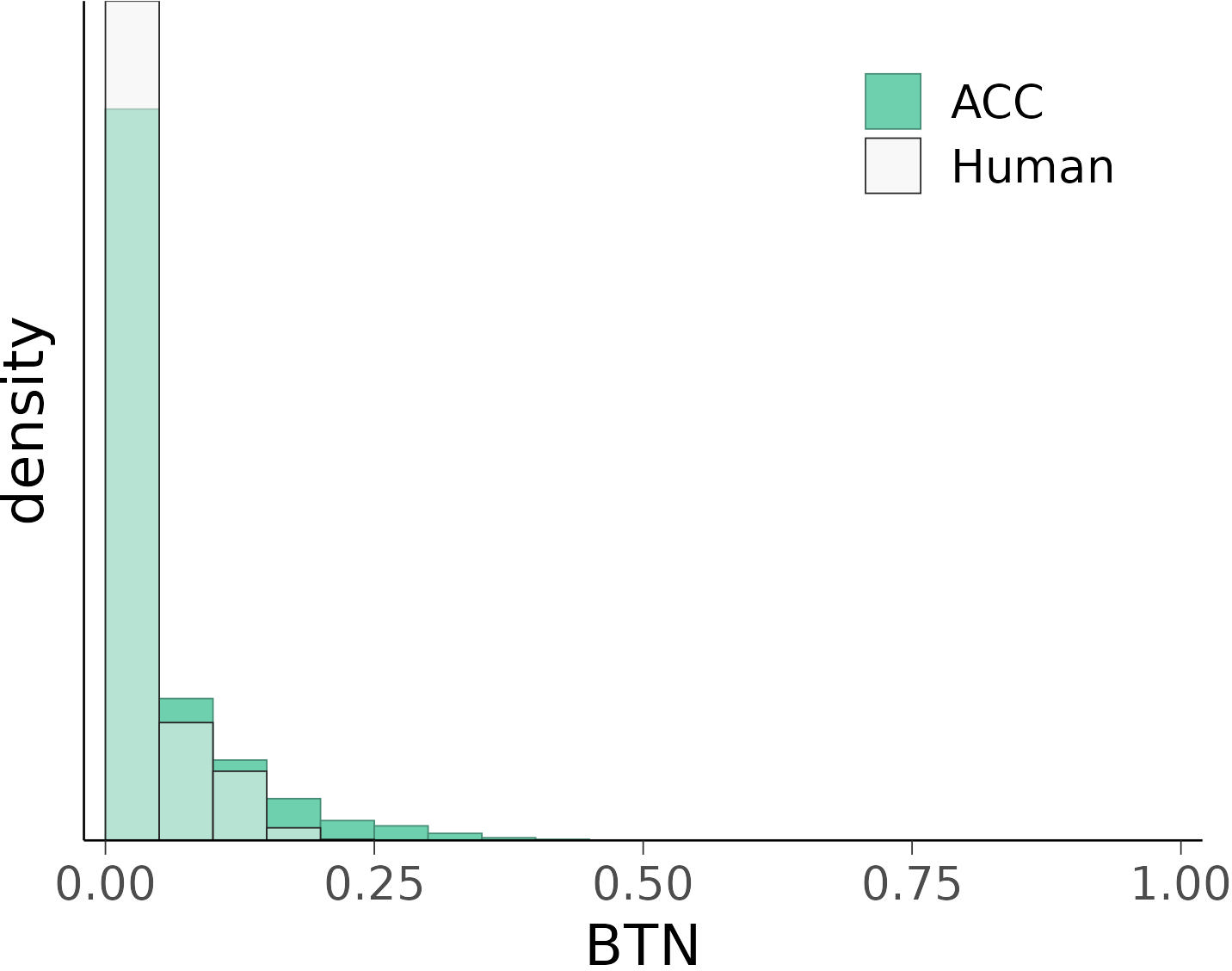
In general, ACC maintained a much shorter headway to the lead vehicle than manual driving (Table 2; Figure 3). The BTN distributions have the same median (equal to 0.0), but the one for ACC has a slightly longer tail (89% percentile: ACC = 0.10; Human = 0.05) compared to manual control. No BTN was greater than 1, regardless of the driving mode (Figure 4).
| Metric | Driving mode | Median | 89% PI |
|---|---|---|---|
| Spacing (m) | Manual | 38.1 | 19.7 – 75.6 |
| ACC | 21.4 | 16.0 – 32.4 | |
| THW (s) | Manual | 2.08 | 1.31 – 3.58 |
| ACC | 1.16 | 0.93 – 1.57 |
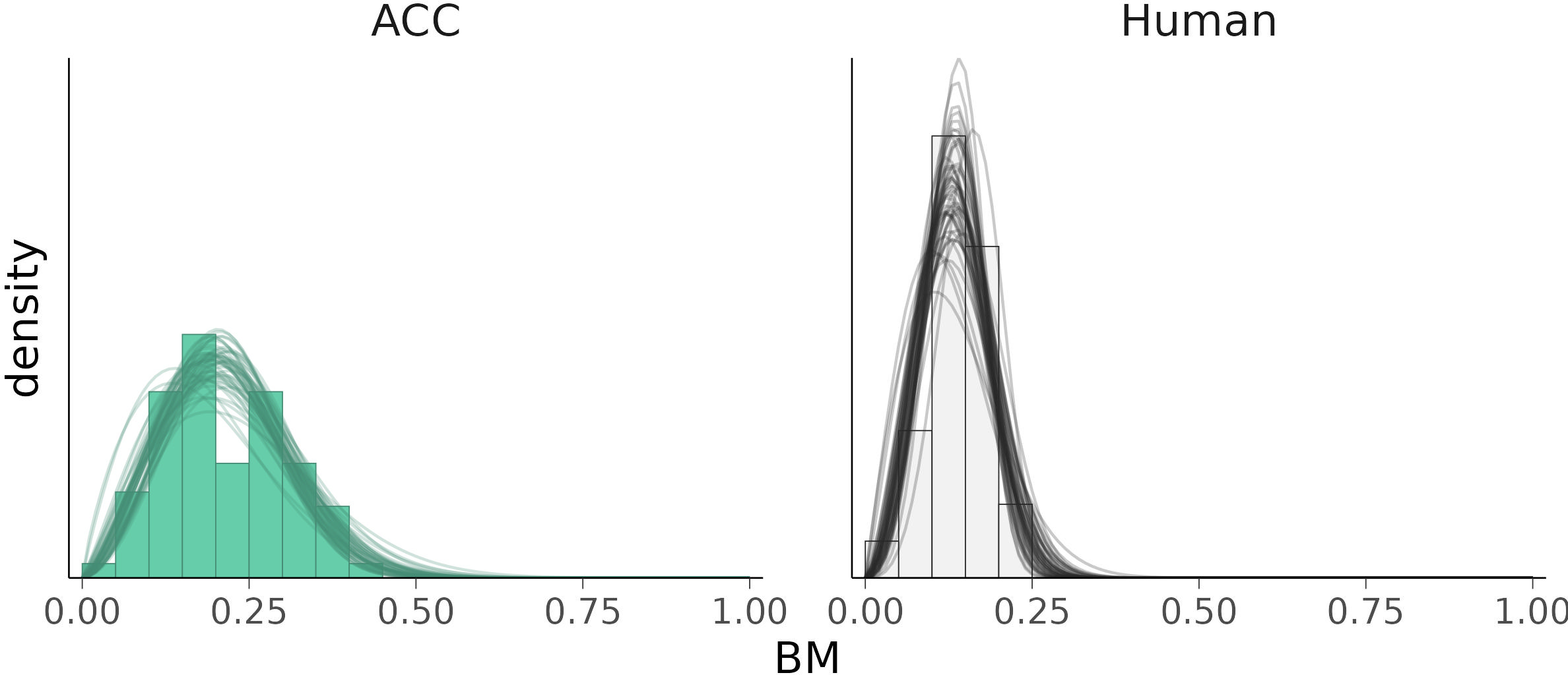
The Bayesian regression model yielded a set of parameters for the Weibull distribution (Table 3) that mimicked the observed BM for each driving mode well (Figure 5). The model was a plausible representation of the empirical data and it could thus be used for extrapolation (i.e., to estimate when and a crash occurs). The BM were higher under ACC than they were under human control (Figure 5). The expected probability of was under ACC. Under manual control, it was many orders of magnitude lower Figure 6). The inverse of this probability is the expected for a crash. Under normal operation of the ACC, according to the model a crash would occur within blocks (equivalent to km), and the lower bound of the PI is blocks km; Figure 7). Under manual control, a crash would occur within blocks km), and the lower bound of the PI is blocks km). As shown in Figure 7, the estimate for RP plateaus quickly in the manual control case.
| Metric | Driving mode | Median | 89% PI |
|---|---|---|---|
| Manual | 0.15 | 0.14 – 0.17 | |
| ACC | 0.24 | 0.22 – 0.26 | |
| Manual | 3.06 | 2.32 – 3.90 | |
| ACC | 2.50 | 2.14 – 2.90 | |
| Manual | 0.14 | 0.12 – 0.15 | |
| ACC | 0.21 | 0.20 – 0.23 |
4. Discussion
Is ACC safe? In general, yes. Based on the data and the model, the results suggest that a potential crash under ACC has a low probability (i.e., a long distance between collisions, in the order of a trillion km). Is ACC safer than manual driving? Sometimes; it depends on what manual driving style we are comparing it to. Our results, which exclude other active safety systems that may be installed in modern cars, indicate that the BTN of a car with ACC alone is higher (i.e., there is higher risk) than that of a car under the control of a cautious human. This finding contradicts the general expectation that ACC is safer than manual driving (Malta et al., 2012, Ch. 4).
4.1. Human control
Previous studies of real-world traffic have found that drivers often follow a lead vehicle too closely; the distance is too short for their typical perception-reaction time. Drivers need more than 1 s to brake (Lamble et al., 1999; Markkula et al., 2016; Summala, 2000; Summala et al., 1998), and the proportion of s can be much higher under human control than with ACC (General Motors Corporation Research and Development Center, 2005, Ch. 8; Malta et al., 2012, Ch. 4; (Varotto et al., 2022), (Morando et al., 2019)). Thus, the potential safety benefit of an ACC that maintains adequate headway is considerable. However, the typical THW in the manual control data in the OpenACC experiment was around 2 s (the value recommended in driving manuals in many European countries Technical Group Road Safety, 2009). Consequently, the safety benefits of ACC in the OpenACC experiment were less pronounced or absent.
Driving is largely a self-paced task; drivers actively adapt their driving to maintain a comfortable safety boundary (Engström & Aust, 2011; Summala, 2007). During routine driving we may follow a vehicle too closely—intentionally because we are in a hurry or unintentionally because we don’t recognize that we are, in fact, too close (Taieb-Maimon & Shinar, 2001). In contrast, professional drivers in a controlled experiment may be more careful than usual because they are aware it is a test. This is one possible reason why our estimates are much more conservative than those of Åsljung, Nilsson, and Fredriksson (2017), despite using a similar method. In addition, Åsljung, Nilsson, and Fredriksson (2017) used a much larger FOT dataset (250.000 km vs. 888 km); they used professional drivers as well, but the data were from real traffic. Their best estimate was km between collisions under manual control, which is close to the rear-end crash frequency in manual driving in motorways in Europe (around km; Dobberstein et al., 2022, para. 6.2). The results of Åsljung, Nilsson, and Fredriksson (2017) are more precise than ours, but their paper also highlights how some modeling decisions can affect the results, particularly with extrapolations over long time horizons. Depending on the method used to fit their models, Åsljung, Nilsson, and Fredriksson (2017) obtained an estimate of – km between crashes. Ultimately, Åsljung, Nilsson, and Fredriksson (2017) chose the model that yielded an estimate closer to the one from crash statistics, but without that reference, we would not know which model is best.
Because of the cautious manual driving and the absence of any external perturbations of the traffic flow, the conditions leading to our results are not the same as those we would observe in regular traffic; the difference is many orders of magnitude vs. km in Dobberstein et al., 2022, para. 6.2). However, despite the small dataset, the model was a good fit to the data (Figures 5, 6, and 7), and the Bayesian model provided a more complete account of uncertainty than maximum likelihood estimates (Coles, 2001, Ch. 9). While the modeling approach shows promise, the available data were not representative of real-world driving behavior. The validity of the results depends on the quality of the input, thus, as with most techniques, agreement with the observed data is a necessary but not sufficient condition to justify long-term extrapolation (Coles, 2001, Ch. 3).
Crashes in manual driving happen for many reasons, including human factors such as inattention and distraction (National Center for Statistics and Analysis, 2022; Singh, 2015). As the professional drivers were careful, it is likely that the data in OpenACC did not include those human crash-contributing factors. In the future, one could supplement the data by simulating driver impairment with different braking parameters (cf. Table 1). For example, when everything else is kept constant, the driver’s response time is the most important parameter in our braking model. Thus, one could include a response time distribution and modulate it for different driver states. In this work, for convenience and reduced computational cost, we assumed that all drivers would recognize a hazard and start braking with a constant reaction time (see also UNECE, 2022, p. 30). However, analyses of crashes in naturalistic driving reveal that drivers’ responses depend on the urgency of the situation and their visual behavior, rather than being a fixed reaction time (Engström et al., 2022; Markkula et al., 2016; Summala, 2000). Moreover, many crashes happen because of a mismatch between drivers’ attention and a rapidly evolving traffic event (Summala, 2000; Victor et al., 2015). Thus, in future work, visual behavior could also be included (see Bärgman et al., 2015), but the computational demand would increase drastically.
4.2. Adaptive Cruise Control (ACC)
There is little information on using EVT for the safety estimation of systems such as ACC. Most of the literature has focused on autonomous emergency interventions (e.g., AEB). Unlike ACC, AEB is usually active by default and is available in most new cars. ACC, instead, is a convenience system that drivers can choose to buy and use (or not). Even though the estimated crash frequency of ACC is higher than defensive manual driving, it is still extremely low—lower than the collision frequency of manual driving on motorways, which are the typical operational design domain of ACC vs. km in Dobberstein et al., 2022, para. 6.2). ACC can, in fact, increase comfort and safety. It is also possible that the higher BM values under ACC in our analysis are the consequence of a deliberate delay in the system intended to prevent discomfort by avoiding adjusting the speed too frequently.
A platoon is an excellent driving situation for gathering data for an EVT analysis, since it provides data on prolonged car-following from multiple vehicles in a single short session. While there is less interference (e.g., due to sensor noise or cut-ins) on a test track than in real traffic, we can assume that ACC operates similarly in both environments. Moreover, the existing sources of interference may become less frequent during normal use as technology improves.
4.3. Brake Threat Number (BTN)
Many different threat metrics can be used as crash surrogates (Li et al., 2021; Westhofen et al., 2022). The most common one—especially in the EVT literature—is the TTC, although previous research has shown that BTN is better than TTC for studying rear-end crashes in manual driving (Åsljung et al., 2017). It is our opinion that proximity measures such as THW and TTC do not provide a useful comparison between automated and manual driving, since they do not account for differences in braking behavior and performance. For example, based on TTC alone, ACC would be less safe than manual driving just because it keeps a shorter headway (Figure 3); such analysis would ignore the fact that ACC is arguably more consistent and rapid at adjusting the distance to the lead vehicle than humans are. The advantage of BTN is that it also incorporates a braking profile, capturing some of the unique features of human control (e.g., brake reaction time; Table 1). Ideally, the brake profile would include additional system interventions (e.g., trigger warnings or autonomous interventions based on the developing lead vehicle conflict) which would not be possible with TTC alone.
Analyses based upon BTN may need to be complemented with other metrics. For example, could be used to estimate the potential injury outcome of a crash (Bärgman et al., 2015; Kusano et al., 2022), since BTN does not provide this information. Unfortunately, exists only when a collision has occurred, so it does not allow extrapolating from near-crashes to crashes, as BTN does. Nonetheless, future work could improve EVT models by including to estimate extreme severity crashes based on observed ones.
5. Conclusions
We estimated the crash risk with ACC compared to human control using EVT and data from a platoon experiment on a test track. EVT offers an advantage over the traditional approach to analyzing crash data since it can be applied to a relatively small dataset collected in a short time. The surrogate safety metric BTN enabled a valid comparison between human control and automation by incorporating specific aspects of braking behavior and performance. Our findings indicate that the crash risk under ACC is much lower than the crash risk for manual driving reported at the European level. However, the crash risk of the human control baseline from our experimental data was even lower; as a result, EVT estimated a higher risk for ACC than for the manual driving. This discrepancy in the evaluation of ACC is due to the defensive driving style in the manual driving data from the OpenACC dataset, which does not reflect the general behavior observed in real traffic. Future work could apply the method presented in this paper to data from more realistic driving situations. This study investigated the safety benefits of manual control and ACC in isolation, since there were no other active safety systems in the car. In addition, human factors such as driver impairment and negative behavioral adaptations to automation, which could be detrimental to safety (Rudin-Brown & Parker, 2004; Smiley, 2000; Victor et al., 2018), were also excluded.
Acknowledgements
This paper is an enhanced version of an earlier work included in Deliverable 4.1 of the EU project MEDIATOR (Chandran et al., 2023). I thank my colleagues at Autoliv Research and members of the Mediator project for their comments and suggestions, as well as Tina Mayberry for the language revision.
CRediT contribution statement
Alberto Morando: Conceptualization, Formal analysis, Methodology, Software, Visualization, Writing—original draft, Writing—review & editing.
Declaration of competing interests
The author is employed at Autoliv (www.autoliv.com), which is a company that develops, manufactures, and sells (among others) vehicle safety products.
Fundings
This research was partially funded by the European Union’s Horizon 2020 research and innovation program under grant agreement No 814.735 (Project MEDIATOR).
Declaration of generative AI use in writing
None.
Ethics statement
None.
Editorial information
Handling editor: Lai Zheng, Harbin Institute of Technology, China
Reviewers: Attila Borsos, University of Győr, Hungary; Zhankun Chen, Lund University, Sweden
Appendix. Optimization problem to compute Brake Threat Number (BTN)
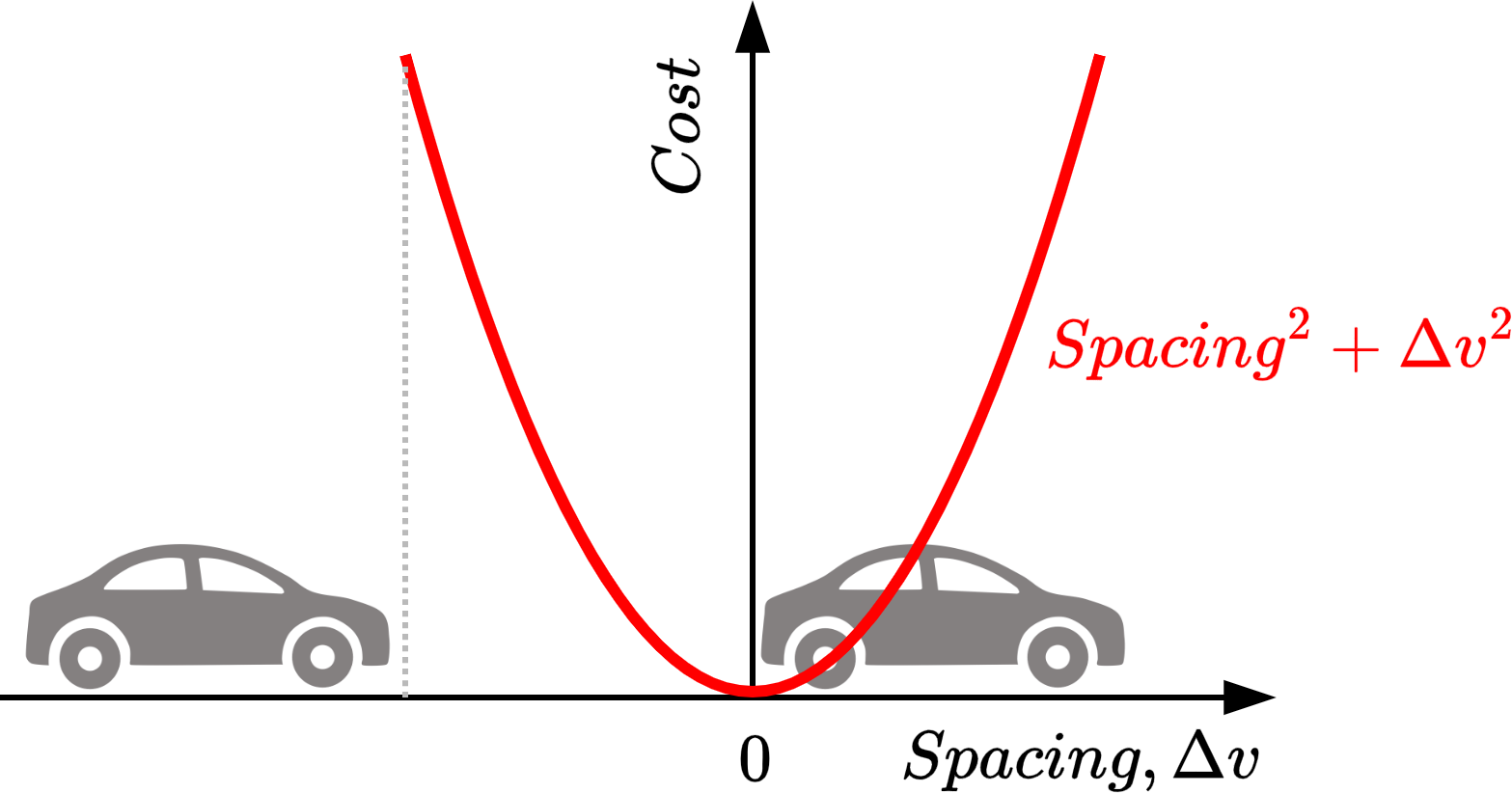
The cost function to be minimized (Figure 8):
where is the spacing between the vehicles and is their relative velocity. The only parameter to optimize (minimize) is :
That is, we want to find the acceleration value that avoids a collision while taking full advantage of the available stopping distance between the following and the leading vehicle.
Velocity traveled distance and spacing are obtained via numerical integration (trapezoidal method) of the kinematic equations for linear motion. The leading vehicle has initial conditions: and acceleration is kept constant, The following vehicle has initial conditions: and the acceleration is modulated according to the brake profile:
For all vehicles, is constrained to positive values: