Built Environment Characteristics and Driving Speed in 30 Km/h Zones: A Dutch National Analysis
Abstract
Road authorities are systematically expanding 30 km/h zones to enhance safety. This requires understanding how built environment characteristics are associated with driving speeds, but only a few studies, typically based on small samples, focus on 30 km/h streets. Using a spatial error model, this study examines the relationship between built environment factors and 85th percentile speeds on 47,000 km of Dutch 30 km/h streets (N=159.000). Driving speed and traffic volume data were estimated using floating car data, while built environment characteristics were collected from public sources.
The results show that higher driving speeds are associated with greater traffic volumes, longer street lengths, closed pavement, separated bicycle tracks, visually marked bicycle lanes, and longer road sections. Features linked to lower driving speeds include curves, speed humps, raised intersections, exit constructions at zone entrances, narrower carriageways, roadside parking, nearby premises, and higher address densities.
Furthermore, the identified interaction effects show that measures like speed humps and raised intersections have greater impacts in high-speed environments (i.e. long and busy streets with closed pavement) but limited effects in low-speed settings. These findings emphasize the need to consider combinations of road design elements and their context-dependent effects to understand driving speed on 30 km/h streets. Out study provides valuable insights into the effectiveness of speed-reduction measures, offering guidance for interventions targeting streets with excessive speeds.
1. Introduction
Speed management plays a central role in the Safe System approach for road safety, as it directly impacts the likelihood and severity of crashes (Aarts & Van Schagen, 2006). For residential areas where motorized traffic is typically mixed with vulnerable road users such as pedestrians and cyclists, a safe speed is no higher than 30 km/h (Tingvall & Haworth, 1999) or even lower according to Lubbe et al. (2022) if the goal is avoid most severe road injuries. Studies show that for pedestrians and cyclists, the risk of death at an impact speed of 50 km/h is about five times higher than at 30 km/h (Hussain et al., 2019; Nie et al., 2015). According to meta-analyses and systematic reviews, area-wide urban traffic-calming schemes in residential areas reduce injury crashes by 25% to 38% (Elvik, 2001; Yannis & Michelaraki, 2024). However, a Dutch study reports that crash reduction is reduced to 15% when speed limits are lowered without extensive infrastructural measures to encourage reduced driving speeds (Schoon, 2000). While reducing speed limits with minimal infrastructure changes allows for quicker implementation (Dissel, 2024), these results underscore the importance of road design and the surrounding environment in sustaining lower driving speeds. Additional benefits of traffic calming are reduced traffic-related noise annoyance (Brink et al., 2022) and increased outdoor physical activity among children and adults (Luo et al., 2021). While a reduced speed limit slightly decreases job accessibility by car, it also enhances bicycle accessibility, which may encourage a shift from driving to cycling (Beek, 2022).
To reap the safety and other benefits, road authorities need an understanding of how a combination road and of environmental characteristics can entice 30 km/h driving speeds within 30 km/h zones. Although several studies have examined driving speeds in urban areas, most used data from streets with speed limits of 40 km/h or higher (Dinh & Kubota, 2013; Jansen et al., 2018; Wang et al., 2006) or a combination of multiple speed limits including some 30 km/h streets (Theeuwes et al., 2024; Van der Kint et al., 2022). Combining different speed limits is necessary for assessing the credibility of a speed limit but may not provide valid insights into driving speeds on roads with a specific limit. For instance for Dutch roads, Theeuwes et al. (2024) found that visually marked bicycle lanes are associated with a lower estimated credible speed limit, while Andriesse (2021) reported an increased speed on busy 30 km/h streets with bicycle lanes. The difference may be due to the purpose and design of each study. While Andriesse (2021) studied the 85th percentile driving speed, participants in the study by Theeuwes et al. (2024), viewed city scenes with and without bicycle lanes and selected credible speed limits from options of 15, 30, 50, and 70 km/h with an equal number of photos per speed limit. The difference may also be attributed to the markings of cycle lanes on otherwise unlined 30 km/h roads, providing visual guidance for drivers. In contrast, 50 km/h roads typically feature centre and edge lines, also in the absence of cycle lanes.
Another limitation of several previous studies is that speed measurements have been made at point locations, typically at midpoints and away from curves (Dinh & Kubota, 2013; Van der Kint et al., 2022). However, this approach may compromise road authorities’ need for knowledge to develop a policy for an entire 30 km/h street. They also need to understand the influence of road and environmental characteristics on driving speed in cohesion. Studies that focus solely on specific road characteristics, such as curves and speed humps near pedestrian crossings (e.g. Fitzpatrick et al., 1997; Gitelman et al., 2017), are valuable for informing guidance but do not offer comprehensive insights into the impact of a combination of characteristics on speed.
To address this knowledge gap, this national study examines the following research question: To what extent are built environment characteristics associated with driving speed in 30 km/h zones in the Netherlands? We focus on the 85th percentile driving speed because it offers valuable insight for traffic safety, highlighting the speeds exceeded by the small group of faster drivers (15%). The paper begins with a literature review to guide the selection of variables (Section 2). The data and methods sections (Sections 3 and 4) detail the dataset and modelling approach. The results section (Section 5) presents key findings, showing how road characteristics influence speed and how these effects vary across different street environments. The discussion (Section 6) contextualizes the results within prior research, explores policy implications, and acknowledges study limitations. Finally, the conclusion (Section 7) summarizes key insights.
2. Literature
2.1. 30 km/h zones in the Dutch context
Dutch road safety policy is founded on the Safe Systems vision called Sustainable Safety which was introduced at the beginning of the nineties (Koornstra et al., 1992; Wegman et al., 2008). Agreement on implementation of the vision was reached in 1998, resulting in the construction of large 30 km/h zones. The so-called access roads in these areas have a residential function where slow traffic and motorized traffic mix, for which 30 km/h is considered a safe speed. To clearly signal the 30 km/h speed limit, no dedicated bicycle infrastructure is built, and no road markings are applied, following the principle of ‘self-explaining roads’ (Theeuwes & Godthelp, 1995). Intersections are preferably yield-to-the-right (CROW, 2021), requiring drivers to slow down at most junctions and check for road users approaching from the right. It also occurs that the right of way is arranged with exit structures: speed hump-like elevated section at the end of a street. Traffic passing the exit construction from the side street has to yield. By 2008, the speed limit on 85% of the roads in built-up areas classified as access roads had been reduced to 30 km/h (Weijermars & Wegman, 2011).
On access roads the volume of motor vehicles should be capped at approximately 3,000 per day, while town centres and shopping areas may accommodate a maximum of 5,000 vehicles daily (Van Minnen, 1999). Road authorities started to reduce speed limits from 50 km/h to 30 km/h on busier roads with a through function in recent years. CROW (2023) has published preliminary design guidelines for this so-called ‘distributor road 30’. We do not focus specifically on these roads that are proportionally still rare (see Andriesse, 2021).
2.2. Theoretical perspectives on driving speed and built environment characteristics
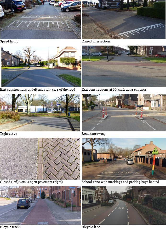
Figure 1 illustrates examples of built environment characteristics observed on 30 km/h roads in the Netherlands that are discussed in this section and included in the study.
Ride comfort
Drivers tend to avoid discomfort due to vertical and lateral accelerations and vibrations. Ride comfort is directly related to vertical accelerations, with 5 m/s² (0.5 g) being a discomfort threshold most drivers avoid (CROW, 2014; Gedik et al., 2019). While measures like speed humps, raised intersections, and exit constructions are designed to induce vertical acceleration at higher speeds, poor road surfaces and uneven pavements can have the same effect. The minimum horizontal curve radii in design guidelines are also based on the upper limit of driver comfort (Said et al., 2009). However, horizontal traffic calming measures, such as chicanes, are generally considered to cause less discomfort than vertical measures like speed humps (Sołowczuk & Kacprzak, 2021), suggesting their speed-reducing effect is better explained by other factors.
Risk and task-difficulty homeostasis
Homeostasis theories assume that drivers monitor and seek to maintain a set level of risk or task difficulty (Fuller, 2007; Wilde, 1982). This theory applies to speed because drivers can reduce risk and task difficulty by lowering their speed (Fuller, 2005). Lewis-Evans & Charlton (2006) found that streets with reduced carriageway width were associated with lower speeds where increased ratings of risk and task difficulty accompany driving. Risk and task complexity are increased at intersections, for which drivers compensate by reduced speeds (Chuna, 2017; Liao et al., 2018). Conversely, speeds are higher the greater the distance between intersections, or in other words, the longer a road section is (Dinh & Kubota, 2013). Drivers also reduce their speed while approaching and driving through a curve or chicane to avoid skidding and manage task-difficulty (Kang et al., 2019; Vos et al., 2021). They chose a lower speed when the radius is smaller and account for the deflection angle of a curve which is better perceived than the radius (Fildes & Triggs, 1985). Reduced speed on roads with on-street parking (Dinh & Kubota, 2013) has also been explained by increased task difficulty and risk compensation (Edquist et al., 2012). Children may cross the road where cars are parked. Likewise, drivers can reduce risks by slowing down when driving through designated school zones with signs or markings (Zhao et al., 2016).
An important factor influencing task difficulty and risk perception in relation to driving speed is the level of visual guidance provided by the road and its surroundings. Roads with edge lines create well-defined lateral boundaries, offering drivers a greater sense of control and stability. This enhanced visual structure fosters confidence and comfort, encouraging drivers to travel faster. Research supports this relationship: subjectively rated effort is lower on roads delineated by edge lines, while driving speeds are higher compared to roads without such markings (Steyvers & De Waard, 2000; Van Driel et al., 2004). Similarly, Kallberg (1993) observed an increase in driving speed following the installation of reflector posts in a Finnish experiment. Reflector posts enhance optical guidance, particularly in darkness, by helping drivers anticipate the road alignment ahead. The absence of delineation on 30 km/h roads may contribute to lower driving speeds. However, roads with bicycle lanes might encourage higher speeds due to the visual guidance provided by the lines and colours of these lanes.
Optical density field of view
According to Gibson (1950), speed perception is strongly determined by optical flow which can be described as the apparent flow of the movement of objects in the visual field relative to the observer. A dense field of view with a high number of objects that contrast with the background slows drivers while a monotonous road environment contributes to higher speeds (Birth et al., 2009; Pretto & Chatziastros, 2006). Characteristics related to optic flow included in speed studies are for instance the density of roadside objects and trees, the presence and height of buildings near the road, and the presence of parked cars along the roadside. (Andriesse, 2021; Dinh & Kubota, 2013; Wang et al., 2006). Note that the impact of regularly placed vertical objects, such as lampposts, on driving speed is difficult to predict. On the one hand, these vertical objects may enhance optic flow, increasing perceived speed and potentially reducing actual speed. On the other hand, their regular placement provides additional visual guidance, which could boost driver confidence and lead to higher speeds. In an experimental study by De Waard et al. (2004) drivers indicated that lampposts made the road’s course clearer, but their driving speed decreased.
Speed impact built environment and urban form via traffic composition and traffic flow
Urban form characteristics, such as population density, built environment density, and land use shape traffic volumes and composition, for instance the mix of pedestrians, cyclists, and the share of vehicles accessing destinations versus the proportion of through traffic (Van Wee, 2009). High densities and the presence of retail areas are linked to increased pedestrian and cycling activity, as well as higher levels of parking movements (Christiansen et al., 2016; Kärmeniemi et al., 2019; Paidi et al., 2022; Schneider & Pande, 2012). In contrast, peripheral industrial zones typically have fewer pedestrians and cyclists.
Traffic flow theory provides insights into how traffic volume affects speed (Daganzo, 1997). As traffic volume nears a road’s capacity, vehicle interactions intensify, reducing speed. This effect becomes more pronounced once capacity is exceeded, resulting in congestion. While lower-order road capacity remains under-researched, two-lane roads are estimated to handle 2,500 to 3,000 vehicles per hour under optimal conditions (CROW, 2013; Kim & Elefteriadou, 2010), translating to tens of thousands of vehicles per day based on the general rule that peak hour traffic accounts for about 10% of daily traffic volume (Van Rij, 2024). Traffic overload at such high volumes is rare on residential 30 km/h roads in the Netherlands (Van Minnen, 1999).
However, traffic composition can influence speeds also at lower volumes (Ewing & Dumbaugh, 2009). Andriesse (2021) observed that higher traffic volumes on 30 km/h roads were associated with increased speeds. This could be explained by a greater proportion of through traffic on busier roads, as these vehicles typically maintain their speed without frequent turning. Also, the presence of pedestrians and cyclists often reduces driving speeds, particularly near intersections or when vehicles need to overtake (Duivenvoorden et al., 2015; Kovaceva et al., 2019). Drivers searching for parking also slow down, potentially reducing the speed of following vehicles (Edquist et al., 2012; Zhu et al., 2020). Additionally, road characteristics impact speed via traffic flow dynamics. For example, separated bicycle tracks and sidewalks may increase driving speeds by reducing the need for overtaking cyclists and pedestrians (Dinh & Kubota, 2013). Conversely, road narrowings can slow traffic, as some drivers wait for oncoming vehicles to pass before proceeding. Yield-to-the-right intersections, common in Dutch 30 km/h zones, may reduce speed as drivers must check the right approach for priority traffic. In contrast, exit constructions on side roads slow vehicles entering or exiting the side roads but signal right of way, thereby increasing the speed of through traffic with priority.
Self-explaining roads
The self-explaining road concept from cognitive psychology (Theeuwes & Godthelp, 1995) suggests that road environments should naturally convey the appropriate expectations including the speed limit. A speed limit needs to be credible and meet the expectations raised by the appearance of the road and its road environment so that drivers are more inclined to comply with them (Schagen et al., 2004). Consistently applied road design features, such as those aligned with the Netherlands’ Sustainable Safety policy (see Section 1.1), play a critical role in shaping these expectations. If other conditions allow, many users will pursue the speed perceived as credible as a target speed. When features typically linked to higher speed limits are present on 30 km/h roads, they increase driving speeds. For example, Andriesse (2021) found driving speed to be increased on busy 30 km/h roads with visually marked bicycle lanes, and multiple driving lanes, all features common on 50 km/h roads.
Integrating Theories on Driving Speed
As suggested by the theories discussed above, driving speed is influenced by several mechanisms involving built environment factors. Built environment factors affect drivers’ perceptions of speed, comfort, risk, and task difficulty. Through a continuous process of calibration, drivers evaluate and adjust these perceptions to align with their desired speed, comfort preferences, risk tolerance, and the level of task complexity they feel capable of managing. This balancing process explains drivers’ unimpeded driving speed. However, external factors, such as delays caused by slower road users, also influence speed behaviour by limiting opportunities for speed choice. Consequently, the calibration process incorporates perceived opportunities for speed choice shaped by traffic flow and potential delays. These are in turn also affected by built environment factors.
Theories also suggest that the impact of built environment factors on speed is influenced by interaction effects. For instance, speed humps, raised intersections, and exit constructions are designed to slow drivers exceeding the 30 km/h limit, with a more substantial effect when other factors encourage speeds above 30 km/h. Similarly, the influence of land use depends on traffic flow and is likely to be more pronounced at higher traffic volumes. In summary, incorporating interaction effects alongside main effects is crucial for this study.
3. Data
We collected data for as many of the variables listed in Section 2 as possible using public sources. All data are linked to the Dutch National Road Database (Nationaal Wegen Bestand, NWB) version January 2024, to create a dataset for statistical analysis. The National Road Traffic Data Portal (NRTP) provides datasets linked to the NWB for many characteristics that are relevant to road safety analyses including analyses on driving speed. The Ministry of Infrastructure and Water Management commissioned the NRTP to collect this data to assist road authorities in measuring Safety Performance Indicators across their road networks.
3.1. Study unit: streets
We conducted our study on a street level, a collection of road sections with the same street name. Firstly, streets are often built at once and subject to similar maintenance, so the street characteristics and surroundings likely match. Secondly, motorists maintain speed when driving straight from one road section to the next.
3.2. Speed data
We utilized the 85th percentile driving speed, as determined by the NRTP using Floating Car Data (FCD) purchased from Be-Mobile for the year 2023. Kijk in de Vegte (2022) compared the FCD estimates to driving speeds measured at 143 locations using loop detectors, road tubes, and radar. On average, the FCD estimate of the 85th percentile speed for FCD road segments of 50 m (or shorter to fit between intersections) only differed by 3 km/h from the loop detector measurements. In this study, we used the dataset provided by NRTP in which the speed data is aggregated to NWB road sections yielding a more accurate speed measure.
For our analysis, the data were further aggregated to the street level by calculating the weighted average of road section speeds, using their respective lengths as weights. An alternative method involves dividing the total street length by the travel time, calculated based on the 85th percentile speed for each road section. These two aggregation methods yield nearly identical results (correlation = 0.997). To ensure consistency with the aggregation approach used for other variables, we adopted the weighted average method. Streets shorter than 50 meters were excluded to ensure that the 85th percentile driving speed estimate was based on data from at least two FCD road segments.
3.3. Infrastructure data
The NRTP provides road feature datasets linked to the NWB via linear referencing (see NDW, 2023). For example, a speed hump is recorded as extending from 34 m to 40 m along a road section with ID 345678. This allowed us to count features such as speed humps and calculate their density per 100 m (representing a fairly high density for these measures) or the proportion of road section length covered by features, such as the percentage of a road section with parking spaces. For parking spaces, the proportion of length refers to the average of the left and right sides of the road meaning that the maximum proportion is 1. A summary of the characteristics and how NRTP collected the data is provided in Table 1.
| Characteristic | Variable expressed as | Road feature dataset NRTP (Dutch name) | Basis |
|---|---|---|---|
| Speed limit | Speed limits (snelheidslimieten) | Inventory and maintenance by road authorities | |
| Speed humps | Density | Speed humps, plateaus and exit constructions (drempels, plateaus en uitritconstructies) | Voluntary registration in large-Scale Topography Registry, and AI recognition on high-resolution aerial photographs within 250 m around primary schools |
| Raised intersection | Density | ||
| Exit construction at road section | Density | ||
| Exit construction along street | Density | ||
| Road narrowing | Density | Road narrowings (wegversmallingen) | Legally required registration in large-Scale Topography Registry |
| Parking space along both sides of the road | Proportion street length | Parking areas (parkeervlakken) | Legally required registration in large-Scale Topography Registry |
| Carriageway width | Average | Carriageway width (wegbreedte) | Legally required registration in large-Scale Topography Registry |
| School address and school zone (road markings and/or signs) | Proportion street length | School zone (schoolzone) | School sites address dataset of Department of education service, national traffic sign database, and AI recognition on high-resolution aerial photographs within 250 m around primary schools |
| Separated carriageways | Proportion street length | Part of national road database (NWB) | Input and maintenance of NWB geometry and features by road authorities and ICT maintenance organisation |
| Road section length | Average | Part of national road database (NWB) | Input and maintenance of NWB geometry and features by road authorities and ICT maintenance organisation |
Aggregation to streets
Infrastructure characteristics were aggregated from road sections to streets by calculating the average of road sections, weighted by their length. For raised intersections that span multiple road sections within a street, the feature was counted once using their unique ID in the road feature dataset for speed humps, plateaus, and exit constructions.
Curves
In 2023, NRTP successfully completed a proof of concept for recognizing curves in the NWB geometry with an angular rotation of at least 30 degrees. A 3 m flat-end buffer was applied along the curves to match with the January 2024 NWB dataset. Curves were classified into two categories: those with angular rotations between 30 and 60 degrees (wide curves) and those with rotations exceeding 60 degrees (tight curves).
Road surface
The July 2024 Large-Scale Topography Registry (Kadaster, 2024b) was used to classify road surfaces into open pavement types such as paver and closed pavement types like asphalt. We excluded speed humps because of their sometimes-differing pavement. A spatial join was performed to identify the pavement type at points spaced every 20 m along each road section, starting 5 m from the beginning and ending no more than 5 m from the road section’s end. The most frequent pavement type was assigned as the pavement type for the entire road section.
Data quality
NRTP has high data quality for many features since they are derived from the Dutch Large-Scale Topography Registry, where governments are legally required to meet prescribed quality standards. However, as including speed humps, raised intersections, and exit constructions in the Large-Scale Topography Registry is voluntary, the quality of this dataset was evaluated (Mieras & Drolenga, 2023). While the dataset contains very few false positives, it is only 82% complete. The distinction between speed humps, raised intersections, and exit constructions is accurate for 92% of the features. Streets within two municipalities were excluded from our study because Mieras & Drolenga (2023) reported that speed humps were not recorded in these areas. Similarly, while the presence of addresses of primary schools is reasonably certain, the quality of the detection of school zone markings has been examined (Rijkswaterstaat, 2023). The feature recognition process on aerial photographs correctly identified 91% of the features it detected (precision). However, it missed about 23% of the total features present, resulting in a recall of 77%, which reflects the overall completeness of the detection process.
3.4. Data on field of view
Building data, mandatory to be collected by each municipality, were extracted from the Basic Register of Addresses and Buildings of September 2024 (version september 2024; Kadaster, 2024a). The area along the carriageway was identified through the NWB line geometry projected at the centre of road areas as registered in the large-Scale Topography Registry, and by using the NRTP pavement width dataset. Flat-end buffers were used along the NWB line geometry, extending half the road width plus 4 m. Before buffering, 10 m at the beginning and end of each section were excluded because of the imprecise location of junctions where road sections start and end. Junctions in NWB still need to be projected in the middle intersection areas in the large-Scale Topography Registry. Since only a narrow parking lane and pavement would fit between the road and any buildings, buildings within these buffers are considered close to the carriageway. The number of buildings within the buffers was counted to determine the density of premises near both sides of the carriageway per 100 m.
3.5. Presence of bicycle infrastructure
In 2024, NRTP partnered with the Dutch Cyclist’s Union to incorporate bicycle infrastructure presence and road access for cyclists from the Cyclist’s Union route database (Fietsersbond, 2024). NRTP linked the Cyclist’s Union data to all road sections with a 30 km/h speed limit based on distance and direction of road sections in both datasets. Since cycling is typically allowed on all 30 km/h roads in the Netherlands, we assumed a road section had separate bicycle tracks if cycling on the carriageway was forbidden, according to the Cyclist’s Union route database. Additionally, visually marked bicycle lanes as recorded by the Cyclist’s Union, were adopted for this study. The proportion of street length with bicycle infrastructure was determined using this information.
3.6. Address density and land use data
We intersected 30 km/h streets with neighbourhood data obtained from Statistics Netherlands (CBS, 2024b) to determine the address density per square km in the area surrounding the street. Further, we calculated the proportion of street length falling within areas designated as shopping zones or industrial areas through land use data from Statistics Netherlands (CBS, 2024a).
3.7. Volumes of motorised traffic
NRTP estimated traffic volumes for all NWB road sections in 2023 using FCD purchased from TomTom. While Be-Mobile data was used for speeds, it did not include probe numbers. The estimates are based on the number of vehicles in the FCD sample (known as probes) and account for variations in coverage across the road network, such as lower coverage on lower-ranked roads (see Hastig, 2024). A comparison with loop detector measurements showed the estimated traffic volume differed less than 10% at 44% of loop detectors and less than 50% at over 90% (NDW, 2024). In this study, we aggregate the average daily traffic volumes of road sections to streets, with the values weighted by the length of each road section.
3.8. Log transformation of traffic volume and street length
According to flow theory, driving speed typically decreases as traffic volume increases. However, Andriesse (2021) found the contrary for even the most busy Dutch 30 km/h streets. This can be explained by the fact that these streets operate well below their capacity. Nevertheless, it is unlikely that speed continues to increase proportionally as traffic volume grows. To account for this tapering effect, we use the natural logarithm of traffic volume as an independent variable. Similarly, while street length is associated with increased driving speed (Rahim & Daniel, 2023) this increase is likely to flatten of as street length grows further. Therefore, both traffic volume and street length are log-transformed. The coefficient in the regression model should be interpreted as the change in the 85th percentile driving speed when these log-transformed variables increase by one unit. This corresponds to the original variables increasing by a factor of e, the base of the natural logarithm ( e≈ 2.72). For example, when a variable increases from 1 to e, its natural logarithm increases from 0 to 1; from e to e2, it increases from 1 to 2, etc.
4. Methods
We used descriptive statistics to summarise the data. To assess possible spatial autocorrelation of speeds on adjacent road sections, we used the Moran’s I statistic and 999 permutations to determine its statistical significance. The Moran’s I ranges from -1 to 1. Positive values indicate positive autocorrelation; negative ones indicate negative autocorrelation. Values above 0.3 are typically deemed as evidence of a strong spatial pattern (Foelske & Van Riper, 2020; O’Sullivan & Unwin, 2014). A buffer was applied around each street to define the spatial weight matrix, allowing overlapping segments to establish adjacency. This approach facilitated the creation of a first-order Queen’s continuity weight matrix, capturing direct spatial dependencies between neighbouring streets. We excluded streets without neighbours.
To assess the multivariate associations using ordinary least squares (OLS), we regressed the response variable (i.e., the 85th percentile driving speed) on the covariates describing the built environment characteristics. Each covariate serves as a control for the others, isolating the effect of each factor. Potential multicollinearity among the covariates was evaluated through the generalised variance inflation factors (GVIF). To ensure comparability across continuous and categorical covariates as well as interaction terms, we used the adjusted GVIF (Gaonkar et al., 2023). As commonly done, we deemed GVIF values >5 as an indication of multicollinearity (Kutner et al., 2004; Valdés-Souto & Naranjo-Albarrán, 2021).
We used the Moran’s I and (robust) Lagrange Multiplier (LM) tests to evaluate whether the OLS residuals face significant spatial autocorrelation. The latter determines an alternative spatially explicit model specification by distinguishing between spatial lag or spatial error models. In our case, the LM test suggested that a spatial error model specification is suitable (Anselin & Berra, 1998). The spatial error model accounts for spatial dependence by capturing spatial autocorrelation in the error term. The model is expressed as follows (Anselin, 1988): Y = βX + λWϵ + ϵ, where Y is the response variable, X is the matrix of independent variables, β is the vector of coefficients for X, W is the spatial weights matrix, λ is the spatial error coefficient, and ϵ is the vector of random errors.
To identify potential interaction variables, we examined correlations between the 85th percentile driving speed and the independent variables. Following Cohen’s (1988) guideline, variables with at least a medium correlation magnitude (i.e., > 0.3) were selected as candidates. These variables are expected to differentiate between low- and high-speed environments, where associations of other variables with speed may vary. These variables were included as interaction terms if their addition improves the model fit, as indicated by a lower Akaike Information Criterion (AIC). Independent variables representing rare characteristics, defined as those occurring on less than 2% of street length, were excluded from interaction terms to reduce the risk of multicollinearity and overfitting.
Analyses were performed in R (R Core Team, 2024), utilising dplyr for data processing, sf for geographic analysis, car for assessing GVIF values, and spdep and spatialreg for spatial analyses. Due to computational limitations in R, we also used GeoDa, designed to handle large datasets in spatial regression analysis efficiently (GeoDa version 1.22) (Anselin et al., 2022; GeoDa, 2024).
5. Results
5.1. Descriptive statistics
Out of the 175,000 30 km/h streets longer than 50 m, we included 159,000 in our study, comprising a total street length of 47,000 km. Streets were excluded due to missing speed data or the absence of neighbouring streets, as the lack of neighbours prevents the incorporation of spatial influences in spatial regression modelling.
Figure 2 shows the distribution of 85th percentile driving speeds by length and frequency. The distribution of 85th percentile driving speeds based on road length is somewhat skewed towards higher values, with fewer streets experiencing low speeds. The distribution based on the number of streets is less skewed, as speeding is less prevalent on shorter streets, which occur more frequently. The average 85th percentile driving speed is 32.2 km/h, with a standard deviation of 4.6 km/h. Moran’s I for the 85th percentile driving speed is 0.32 (p = 0.001), indicating positive spatial autocorrelation, likely due to drivers maintaining speeds as they move from one street to another.
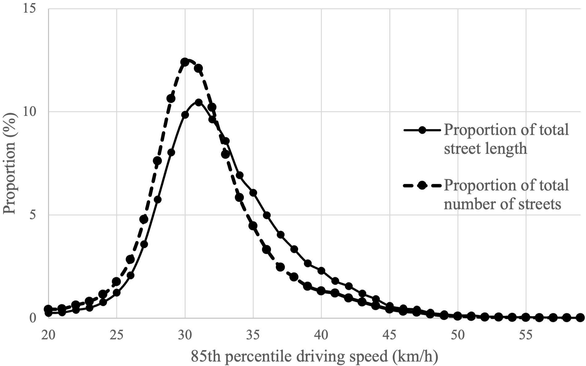
Table 2 presents descriptive statistics, including the mean, standard deviation, and correlations of all variables with the 85th percentile driving speed. Variables are listed in descending order of the absolute value of their correlations. Notably, the proportion of street length with closed pavement, the logarithm of motor vehicles per day, and the logarithm of street length exhibit positive correlations exceeding 0.3. Conversely, the proportion of road section length within the total street length with a school address is the only variable with a correlation that is not statistically significant. The averages reveal substantial variation in the frequency of characteristics. For instance, raised intersections, with an average density of 0.28 per 100 m, are relatively common. In contrast, features such as cycle tracks and school zones, with an average proportion of street length of just 1%, can be considered rare.
| Variable | Mean (SD) | Correlation with speed | |
|---|---|---|---|
| 85th percentile driving speed | 32.20 (4.63) | ||
| Closed pavement (prop. length) | 0.25 (0.41) | 0.37 | *** |
| Logarithm traffic volume (100 motor vehicles per day) | 0.64 (1.12) | 0.33 | *** |
| Logarithm total street length (100 m) | 0.80 (0.73) | 0.31 | *** |
| Density per 100 m of premises within 4 m of the carriageway | 2.42 (4.12) | 0.25 | *** |
| Density of tight curves per 100 m with a rotation angle over 60° | 0.17 (0.37) | 0.24 | *** |
| Visually marked bicycle lane (prop. length) | 0.02 (0.12) | 0.22 | *** |
| Separated bicycle track (prop. length) | 0.01 (0.10) | 0.22 | *** |
| Addresses per square km (x 1.000) | 1.53 (1.36) | 0.20 | *** |
| Average road section length (100 m) | 0.96 (0.64) | 0.20 | *** |
| Parking spaces along the road (prop. length) | 0.18 (0.19) | 0.18 | *** |
| Carriageway width (m) | 5.12 (1.04) | 0.16 | *** |
| Density of wide curves per 100 m with a rotation angle over 30-60° | 0.17 (0.34) | 0.13 | *** |
| Industrial zone (prop. length) | 0.02 (0.13) | 0.13 | *** |
| Exit construction density per 100 m on the street | 0.06 (0.22) | 0.09 | *** |
| Speed hump density per 100 m | 0.22 (0.42) | 0.09 | *** |
| Separated carriageways (prop. length) | 0.02 (0.12) | 0.07 | *** |
| Shopping area (prop. length) | 0.03 (0.14) | 0.06 | *** |
| Raised intersection density per 100 m | 0.28 (0.47) | 0.04 | *** |
| Exit construction density per 100 m along the street | 0.03 (0.15) | 0.04 | *** |
| School zone with signs and/or markings (prop. length) | 0.01 (0.07) | 0.03 | *** |
| Road narrowing density per 100 m | 0.07 (0.24) | 0.02 | *** |
| School address at road section (prop. length) | 0.01 (0.06) | 0.00 |
5.2. Regression analysis
We began the regression analysis with an OLS model on the 85th percentile driving speed, including all variables listed in Table 2 but without interaction terms. All GVIF values remained below 1.5, indicating that multicollinearity is unlikely. Because the model showed residual spatial autocorrelation (Moran’s I =0.24, p<0.001) and was supported through the LM test (p<0.001), we fitted a spatial error model. The overall model fit was with a pseudo-R2 of 46% better than the OLS model with an R2 of 39%; further supported through the AIC scores (AICSER= 804106, AICOLS= 816480). The spatial error coefficient λ was 0.32 suggesting moderate spatial dependence in the error terms. Table 3 presents the main results of the spatial error model for 85th percentile driving speed. The coefficients and confidence intervals provide insight into how each variable is related to driving speed.
| Variable | Estimate (95% CI) | |
|---|---|---|
| Intercept | 30.11 (29.99 to 30.22) | *** |
| Closed pavement (prop. length) | 2.17 (2.12 to 2.22) | *** |
| Logarithm traffic volume (100 motor vehicles per day) | 0.73 (0.71 to 0.75) | *** |
| Logarithm total street length (100 m) | 0.78 (0.75 to 0.80) | *** |
| Density per 100 m of premises within 4 m of the carriageway | -0.09 (-0.10 to -0.09) | *** |
| Density of tight curves per 100 m with a rotation angle over 60° | -2.02 (-2.07 to -1.97) | *** |
| Visually marked bicycle lane (prop. length) | 3.66 (3.51 to 3.80) | *** |
| Separated bicycle track (prop. length) | 5.22 (5.03 to 5.41) | *** |
| Addresses per square km (x 1,000) | -0.43 (-0.45 to -0.41) | *** |
| Average road section length (100 m) | 0.52 (0.49 to 0.55) | *** |
| Parking spaces along the road (prop. length) | -1.24 (-1.34 to -1.13) | *** |
| Carriageway width (m) | 0.30 (0.28 to 0.32) | *** |
| Density of wide curves per 100 m with a rotation angle over 30-60° | -1.37 (-1.42 to -1.32) | *** |
| Industrial zone (prop. length) | 1.76 (1.59 to 1.92) | *** |
| Exit construction density per 100 m on the street | -0.75 (-0.83 to -0.68) | *** |
| Speed hump density per 100 m | -0.66 (-0.70 to -0.62) | *** |
| Separated carriageways (prop. length) | 0.71 (0.56 to 0.86) | *** |
| Shopping area (prop. length) | -0.94 (-1.09 to -0.79) | *** |
| Raised intersection density per 100 m | -0.07 (-0.11 to -0.02) | ** |
| Exit construction density per 100 m along the street | 0.64 (0.53 to 0.76) | *** |
| School zone with signs and/or markings (prop. length) | 0.42 (0.18 to 0.65) | *** |
| Road narrowing density per 100 m | -0.22 (-0.29 to -0.15) | *** |
| School address at road section (prop. length) | -0.23 (-0.49 to 0.03) |
The variables are presented in Table 3 in the same order as in Table 2. The direction of all regression coefficients aligns with the direct correlations reported in Table 2. Once again, the proportion of street length with a school address is the only variable not statistically significant. The following variables are associated with higher 85th percentile driving speeds: closed pavement, higher traffic volumes, longer street lengths, bicycle lanes and tracks, longer average road section lengths, wider carriageway widths, a greater proportion of street length through industrial zones, separated carriageways, exit constructions on side roads, and a greater proportion of street length through school zones with signs and/or markings. The association with school zones is weak, showing only a 0.4 km/h increase in speed for streets that are entirely within such zones. Nonetheless, this positive association is contrary to our expectations, as school zones are typically designed to reduce speed.
In contrast, the following variables are associated with lower 85th percentile driving speeds: premises close to the carriageway, curves (especially tight curves), high address density, parking spaces along the street, exit constructions on the street, speed humps, raised intersections, and a greater proportion of street length through shopping areas. Although road narrowing density also shows a statistically significant negative association, the effect is negligible with only 0.2 km/h lower speed per road narrowing per 100 m.
5.3. Regression analysis with interaction effects
Interaction terms to be included
At the end of section 2.2 we hypothesized that the impact of built environment factors on speed is influenced by interaction effects. We considered including interaction terms for the three variables with correlations over 0.3 with 85th percentile driving speed (see Table 2) that distinguish between a low and high speed environment where the effect size of other independent variables may vary. Each variable, when added as an interaction effect, improves the model fit compared to the model of the previous section without interaction terms: length proportion with closed pavement (1.5% higher pseudo-R2; 4185 lower AIC), the logarithm motor vehicles per day (2.4% higher pseudo-R2; 6695 lower AIC), and the logarithm of street length (2.5% higher pseudo-R2; 7169 lower AIC). The largest improvement is achieved with all three two-way interaction effects (4.2% higher pseudo-R2; 12118 lower AIC). All GVIF’s remained under 2 and that model was therefore chosen for the analysis with interaction effects.
Main effects
Table 4 presents the main results of the spatial error model for 85th percentile driving speed. Similar to the model without interactions, the spatial error coefficient λ was 0.32 suggesting moderate spatial dependence in the error terms. The second column of Table 4 presents the main effects, which describe associations for streets where the three interaction terms are zero. For most variables, the direction of the main effect matches those of the model without interactions (see Table 3) but the magnitudes of the effects are smaller. For raised intersections and shopping areas, there is not even a significant main effect.
| Interaction effects (95% CI) | ||||||||
|---|---|---|---|---|---|---|---|---|
| Variable | Main effects (95% CI) | Traffic volume | Street length | Closed pavement prop. | ||||
| Intercept | 30.25 (30.10 to 30.40) |
*** | ||||||
| Closed pavement (prop. length) | 2.90 (2.64 to 3.16) |
*** | 0.55 (0.50 to 0.59) |
*** | -0.07 (-0.13 to -0.01) |
* | ||
| Logarithm traffic volume (100 motor vehicles per day) | 0.24 (0.16 to 0.33) |
*** | ||||||
| Logarithm total street length (100 m) | 1.18 (1.04 to 1.32) |
*** | 0.35 (0.33 to 0.37) |
*** | ||||
| Average road section length (100 m) | 0.14 (0.08 to 0.19) |
*** | -0.04 (-0.06 to -0.01) |
** | 0.26 (0.22 to 0.29) |
*** | 0.08 (0.01 to 0.14) |
* |
| Speed hump density per 100 m | -0.28 (-0.35 to -0.22) |
*** | 0.02 (-0.02 to 0.07) |
-0.46 (-0.53 to -0.40) |
*** | -0.60 (-0.71 to -0.48) |
*** | |
| Raised intersection density per 100 m | 0.02 (-0.03 to 0.07) |
-0.01 (-0.05 to 0.03) |
-0.19 (-0.25 to -0.14) |
*** | -0.55 (-0.66 to -0.44) |
*** | ||
| Exit construction density per 100 m on the street | -0.41 (-0.50 to -0.32) |
*** | -0.36 (-0.42 to -0.29) |
*** | -0.44 (-0.56 to -0.32) |
*** | -0.60 (-0.83 to -0.37) |
*** |
| Exit construction density per 100 m along the street | 0.35 (0.18 to 0.51) |
*** | 0.14 (0.05 to 0.23) |
** | 0.19 (0.04 to 0.33) |
* | 0.02 (-0.26 to 0.30) |
|
| Road narrowing density per 100 m | -0.17 (-0.26 to -0.07) |
*** | 0.08 (0.01 to 0.14) |
* | -0.23 (-0.34 to -0.13) |
*** | 0.23 (0.05 to 0.41) |
* |
| Density of wide curves per 100 m with a rotation angle over 30-60° | -0.72 (-0.79 to -0.66) |
*** | -0.14 (-0.18 to -0.09) |
*** | -1.12 (-1.20 to -1.05) |
*** | -0.31 (-0.45 to -0.18) |
*** |
| Density of tight curves per 100 m with a rotation angle over 60° | -1.42 (-1.47 to -1.36) |
*** | -0.17 (-0.21 to -0.12) |
*** | -1.59 (-1.66 to -1.51) |
*** | -0.47 (-0.62 to -0.33) |
*** |
| Carriageway width (m) | 0.23 (0.20 to 0.25) |
*** | 0.09 (0.08 to 0.10) |
*** | -0.01 (-0.03 to 0.02) |
-0.10 (-0.14 to -0.05) |
*** | |
| Density per 100 m of premises within 4 m of the carriageway | -0.06 (-0.07 to -0.05) |
*** | -0.02 (-0.03 to -0.02) |
*** | -0.06 (-0.06 to -0.05) |
*** | -0.08 (-0.09 to -0.06) |
*** |
| Addresses per square km (x 1,000) | -0.25 (-0.28 to -0.23) |
*** | -0.08 (-0.09 to -0.07) |
*** | -0.08 (-0.10 to -0.06) |
*** | -0.26 (-0.30 to -0.21) |
*** |
| Shopping area (prop. length) | -0.01 (-0.21 to 0.18) |
-0.56 (-0.66 to -0.46) |
*** | -0.27 (-0.46 to -0.08) |
** | -0.26 (-0.65 to 0.13) |
||
| Separated carriageways (prop. length) | 0.60 (0.45 to 0.74) |
*** | ||||||
| Visually marked bicycle lane (prop. length) | 2.11 (1.96 to 2.26) |
*** | ||||||
| Separated bicycle track (prop. length) | 3.65 (3.46 to 3.84) |
*** | ||||||
| Parking spaces along the road (prop. length) | -0.76 (-0.90 to -0.62) |
*** | ||||||
| School address at road section (prop. length) | -0.21 (-0.45 to 0.04) |
|||||||
| School zone with signs and/or markings (prop. length) | 0.33 (0.10 to 0.55) |
** | ||||||
| Industrial zone (prop. length) | 1.80 (1.64 to 1.96) |
*** | ||||||
Interaction effects
The interaction effect coefficients in Table 4 represent the effects of the independent variables in response to a greater length share with closed pavement, traffic volume and street length. To aid interpretation of the magnitude and direction of these effects, Figure 3 visualizes the combined main and interaction effects for two street types:
-
Low-speed environment: open pavement, 100 motor vehicles per day and a street length of 100 m—values close to the 15th percentile of the distributions of the latter two variables. These associations for these streets represent the main effects in the model.
-
High speed environment: closed pavement, 450 motor vehicles per day and a street length of 500 m—both values close to the 85th percentile of their respective distributions. These associations for these streets combine the main effects with interaction effects.
When other variables are equal to zero (e.g. zero densities and length proportions), the model estimates a speed difference of approximately 7 km/h between the low- and high-speed environments. All effects are expressed in Figure 3 in the same units as Table 3, except for premises close to the carriageway, which is presented as 10 per 100 m to highlight an environment where this feature is prevalent.
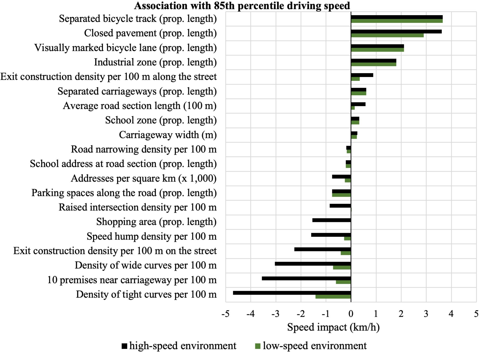
The direction of effects differs minimally between low- and high-speed environments. However, interaction effects show that most associations are significantly stronger in high-speed environments, with weaker or negligible effects in low-speed environments. For example, the effects of average road section length, raised intersections, and shopping areas are substantial in high-speed environments but minimal in low-speed ones.
The key takeaway from the model with interaction-effects is that speeds are higher on 30-km/h streets with closed pavement, higher traffic volumes, and longer lengths, and that these features amplify the impact of other variables. On such streets, speed-inhibiting features have a stronger effect than average, including curves, speed bumps, raised intersections, shopping areas, high address density, premises close to the carriageway, and parking spaces. Fewer speed-enhancing features were included in the interaction effects, but those present had a stronger impact in high-speed environments, for instance, average road section length and exit constructions along the street.
Traffic volume, street length, and closed pavement all contribute in the same direction to the overall association (main plus interaction effects) between the covariates and the 85th percentile driving speed. Based on the magnitude of the interaction effects, street length appears to have a slightly stronger influence on the overall associations than closed pavement and traffic volume, though all three are substantial.
6. Discussion
This study aimed to answer the question: To what extent are built environment characteristics associated with driving speed in 30 km/h zones in the Netherlands? For nearly all variables, the associations with 85th percentile driving speed are broadly consistent with the expectations described in Section 2. The following variables are associated with higher 85th percentile driving speeds: closed pavement, higher traffic volumes, longer street lengths, bicycle lanes and tracks, longer average road section lengths, wider carriageway widths, a greater proportion of street length through industrial zones, separated carriageways, and exit constructions on side roads. In contrast, the following variables are associated with lower 85th percentile driving speeds: curves (especially tight curves), premises close to the carriageway, parking spaces along the street, exit constructions on the street, speed humps, raised intersections, high address density, and a greater proportion of street length through shopping areas. These insights are not only relevant for understanding driving behaviour but also offer valuable guidance for practitioners designing and modifying road environments.
However, a few factors showed only weak relationships with 85th percentile speed. After controlling for other model variables, the presence of school zone signage and markings did not seem to reduce speed. This could suggest that these signals are not sufficiently conspicuous, or that drivers only slow down around school opening and closing times when parking movements naturally reduce speeds. In contrast, our focus was on the all-day average 85th percentile driving speed. The impact of road narrowings on speed was significantly smaller than that of other speed inhibitors like speed humps and raised intersections. This may be due to the infrequency with which drivers encounter oncoming vehicles on 30 km/h streets, meaning they rarely need to reduce speed for oncoming traffic. In such cases, drivers can generally maintain their speed with minimal adjustments. The effect of carriageway width on speed was also relatively small. This should be interpreted with caution, as many streets in our dataset allow on-street parking where no designated parking bays are available, potentially altering the effective width from the measured carriageway width. The effect of carriageway width might have been more pronounced had we been able to include a variable for on-street parking.
The results closely align with findings from the few prior studies that have examined factors influencing speeds on 30 km/h streets. Dinh & Kubota (2013) found higher 85th percentile speed for longer street sections, higher roadside object density, and carriageway width. Andriesse (2021) studied 85th percentile driving speed on busy 30 km/h streets with a flow function. Consistent with our findings on busy 30 km/h streets, he observed lower speeds on streets that pass through shopping areas and have frequent parking movements, and higher speeds on streets with asphalt pavement, bicycle lanes, and higher traffic volumes. While our study found lower speeds on roads with premises close to the carriageway, Andriesse identified a similar trend on streets bordered by higher buildings. That the number of variables with a significant relationship with 85th percentile speed is lower in those studies is probably due to their smaller sample size: 85 selected street sections in the study by Dinh & Kubota (2013) and 179 streets in the study by Andriesse (2021) versus 159,000 streets in the current study.
6.1. Exit construction and raised intersections
The association between the 85th percentile driving speed within a 30 km/h zone and the two intersection measures—exit constructions and raised intersections—seems complex. Our results indicate that a density of one speed hump per 100 m is associated with a greater speed reduction than one raised intersection on the same street. However, a raised intersection not only benefits the street where it is located but also has an impact on the intersecting streets, broadening its effect. Within a 30 km/h zone, raised intersections can achieve a comparable reduction in the 85th percentile speed as speed humps. A raised intersection is also a valuable speed-reducing measure as it lowers speed at a location where road users interact.
Exit structures are also applied at intersections. On the street with the exit structure, speeds typically decrease. However, traffic on adjacent streets, where priority is granted, often experiences an increase in speed. When both the street with the exit structure and the adjacent priority street are quiet and short, these effects tend to offset each other. The overall effect is generally a speed reduction when both are longer or busier streets with closed pavement. However, longer streets are more frequently prioritised due to exit structures on quieter side streets, which can lead to an increase in average speeds within the 30 km/h zone: according to our results the speed increase on long, asphalt priority roads outweighs the speed reduction on short, open-pavement streets with exit structures. In the Dutch context, many exit structures connect 30 km/h streets to 50 km/h priority roads. In these cases, the exit structure slows traffic on the 30 km/h street, while drivers on the 50 km/h road maintain their speed due to priority signage, also without an exit structure. This configuration usually reduces speed within the 30 km/h zone. In summary, exit structures are particularly effective for lowering speed when used as entrances to 30 km/h zones.
6.2. Interaction effects
Many factors on 30 km/h streets make a difference particularly when a street entices high driving speeds due to its greater length, high traffic volume and closed pavement. For measures designed to cause vertical acceleration like speed humps, raised intersections, and exit constructions, this can be explained by the associated discomfort among drivers remaining under a threshold acceptable for drivers while driving no faster than 30 km/h. We also observe an interaction with the presence of buildings close to the road and parking bays, which often coexist with parked vehicles. Through optic flow, these elements contribute to a perception of higher speed. However, we lack a specific explanation for why this perception would be stronger in certain environments, as suggested by the interaction effect.
The various similar interaction effects can be summarised as creating a greater difference on long, busy streets with closed pavement. Conversely, they translate to less difference on short, quiet streets with open pavement. This may be explained by the theory of self-explaining roads, along with 30 km/h being perceived as relatively slow and as a lower threshold for the fastest 15% of motorists. Considering the length of road sections, we also observe this pattern in the distribution of the 85th percentile driving speed, where the range of speeds above 30 km/h is greater than that below 30 km/h. If a street conveys characteristics of a 30 km/h zone—open pavement, quiet and short—this 30 km/h speed might represent what these motorists perceive as an appropriate target, thereby diminishing the effects for those in our model in such a low-speed environment.
6.3. Study limitations and recommendations for future research
A key strength of this study is its large sample size, which provides substantial statistical power. However, its cross-sectional design limits our ability to establish causal relationships. For example, speed-reduction measures might be implemented in response to high driving speeds, making these measures more frequent in areas associated with higher speeds. Unless all relevant conditions are statistically controlled for, this may lead to an underestimation of the measures’ true effects (Elvik, 2011). In contrast, a before-after study would avoid this limitation by comparing speed in the same locations before and after an intervention.
Another limitation is the inconsistent data quality, which may have affected the effect estimates. For instance, we know that the database of speed humps, exit constructions, and raised intersections is 82% complete (Mieras & Drolenga, 2023). Such incomplete data can blur the estimated effects, potentially underestimating the true effect. We recommend further investigation into data quality and repeating a similar study in the future with improved data, both in the Netherlands and internationally, to enable comparisons. For example, in the Netherlands, NRTP is working to enhance the quality of the aforementioned database, which will allow for a more accurate assessment of the effects of speed humps, exit constructions, and raised intersections.
Finally, we assume that the measures are implemented uniformly. However, in practice, there is variation. For example, speed humps differ in height, and we would ideally account for such variations in our model as taller humps are likely to be more effective at reducing speed. This will become feasible with the collection of more detailed data, which should therefore be considered.
New research questions emerge based on the needs of road authorities. Road authorities are increasingly lowering speed limits to 30 km/h on busier through roads. In response, CROW (2023) has published preliminary design guidelines for these so-called ‘distributor roads 30.’ Research is needed to assess how effectively these guidelines encourage drivers to adhere to the 30 km/h speed limit. As more such roads are implemented, opportunities for research will also increase.
This study has shown the value of examining speed behaviour for roads with a specific speed limit. Similar large-scale speed research is recommended for roads with other speed limits. In the Netherlands, while 30 km/h roads serve as access roads in urban areas, 60 km/h roads function as access roads in rural areas, where cyclists are typically mixed with motorized traffic. From a road safety perspective, investigating speed behaviour on these roads in relation to their characteristics is equally important as on 30 km/h roads.
6.4. Practical application
In addition to understanding the relationship between measures and driving speed, our study suggests several options for practice. Despite the good coverage of floating car data for 30 km/h roads, there are roads where insufficient data is available or cannot be appropriately linked to the national road database. Driving speed on these streets can be estimated using a model like the one developed in this study. The model could also be applied to evaluate the design of expanding residential areas, where opportunities to adapt the built environment are most abundant. Furthermore, a modelling approach for 85th percentile driving speed, such as the one used in the current study, could be employed to visualize and quantify potential speed reductions from various measures for existing streets, providing valuable insights to inform road safety policy.
7. Conclusion
This study analysed the relationship between built environment factors and 85th percentile driving speeds on 30 km/h streets using a spatial error model. Our findings reveal that higher driving speeds are associated with greater traffic volumes (within the range common on Dutch 30 km/h streets), longer street lengths, closed pavement, separated bicycle tracks, visually marked bicycle lanes, and longer road sections. Features linked to lower driving speeds include curves (especially tight curves), speed humps, raised intersections, exit constructions at zone entrances, narrower carriageways, roadside parking, nearby premises, and higher address densities. Furthermore, the identified interaction effects show that most associations with built environment factors are greater in high-speed environments (i.e. long and busy streets with closed pavement) than in low-speed settings. These findings emphasize the need to consider combinations of road design elements and their context-dependent effects to better understand driving speed on 30 km/h streets.
CRediT contribution statement
Paul Schepers: Conceptualization, Formal analysis, Investigation, Methodology, Writing—original draft, Writing—review & editing. Werner van Loo: Conceptualization, Data curation, Validation. Wouter Mieras: Conceptualization, Methodology. Hans Drolenga: Conceptualization. Dick de Waard: Conceptualization. Marco Helbich: Methodology, Writing—review & editing.
Data availability
Data used for this study can be downloaded or requested from:
-
Infrastructure: https://downloads.rijkswaterstaatdata.nl/wkd/
-
Land use: https://www.cbs.nl/nl-nl/dossier/nederland-regionaal/geografische-data
-
Driving speed: https://www.ndw.nu/ndw/themas/verkeersveiligheid/risicogestuurd-verkeersveiligheidsbeleid/snelheidsgegevens-voor-verkeersveiligheid
-
Traffic volume: https://www.ndw.nu/ndw/themas/verkeersveiligheid/risicogestuurd-verkeersveiligheidsbeleid/verkeersintensiteiten-voor-verkeersveiligheid
Declaration of competing interests
The authors have no conflict of interests to declare.
Declaration of generative AI use in writing
This research paper has benefited from the use of ChatGPT, a generative AI tool, to enhance the readability and language of the text. The AI was utilized exclusively to improve clarity, coherence, and grammar, with all substantive content, analysis, and interpretations remaining the sole responsibility of the authors.
Ethics statement
This study did not require formal ethical approval, as it exclusively utilized existing open-source data. The data analysed were publicly available and did not include any personally identifiable information or sensitive content. All research activities adhered to ethical standards for the use of secondary data.
Funding
This work did not receive external funding.
Editorial information
Handling editor: Haneen Farah, Delft University of Technology, the Netherlands
Reviewers: Rune Elvik, Institute of Transport Economics, Norway; George Yannis, National Technical University of Athens, Greece