Safety Performance Functions in a Road Environment With Automated Vehicles
Abstract
The reduction of road fatalities can be achieved by intervening in various aspects, including infrastructure, transportation policy, vehicles, and driver behavior. One of the most promising solutions to solve this issue is to rely on Automated Vehicles (AVs), which can prevent human errors, which account for most crashes. However, the impact of AVs on road safety is still unquantifiable. The reason resides in a lack of observed data, as well as in the uncertainty about AV introduction on roads and their interaction with other vehicles and users. In this paper, a methodology to predict the impact of AVs is proposed, relying on Safety Performance Functions (SPFs). An ad hoc SPF for AVs has been developed just for multivehicle crashes, based on a set of market penetration rates, to propose a mathematical model that can include recent technological innovations in road traffic and be adapted to other contexts. Considering the area of the Province of Bari and three different time horizons, crashes were simulated with the presence of AVs in different traffic scenarios. The proposed scenarios were taken from extensive literature studies about the deployment of AVs. The SPF for the predicted crashes was developed by adding one coefficient that considers the presence of AVs to the baseline equation, controlling for the road geometry. The fitted models show a satisfactory goodness-of-fit, based on different metrics, including CuRe (Cumulative Residuals) plots.
1. Introduction
Safety Performance Functions (SPFs) aim to predict the frequency of crashes based on several road, traffic, and environment-related factors. The use of SPFs in routine crash prediction practice, fostered by several decades of research on crash prediction models, is due to the Highway Safety Manual (HSM), which provides an operational framework for each step of the road safety management process. This process requires continuous monitoring of the reference road network, improved site selection, identification, and assessment of possible interventions (National Academies of Sciences, Engineering, and Medicine, 2010). These operations are closely linked to quantifying the number of crashes and the people involved in fatal and injury crashes that occurred during a given period, considering past (observed data) and future periods (predictions for different project scenarios). The baseline equation of SPFs, only considering risk exposure variables, can be defined as follows:
Where:
-
is the predicted mean crash frequency for the SPF related to basic conditions, for a generic road element, segment or intersection (crashes/year)
-
is the annual average daily traffic (vehicles/day)
-
is the length of the site (km)
-
are coefficients to be estimated through the model regression.
This baseline equation can be modified to consider specific cases and different environmental conditions by means of Crash Modification Factors (CMFs). The SPF is multiplied by the CMFs, which consider differences between the geometric and functional conditions of the site under analysis and the baseline conditions of the HSM. International literature also reports on crash prediction models which already include several influential variables, besides exposure measures, in a full model (see e.g., Ambros et al., 2018).
It is evident, however, that the reliability of crash predictions depends on the availability of local SPFs or at least of suitable calibration coefficients for the types of roads under examination. The transferability of SPFs to other contexts has been found to be a suitable approach for reliable safety predictions (Farid et al., 2016; Intini et al., 2019; Lee et al., 2019). This may help in estimating safety performances because the development of a local SPF requires several years of observed crash data and modelling effort.
SPFs are developed for specific road elements, such as intersections (Essa et al., 2019; Intini et al., 2021) or segments (Cafiso et al., 2018; Intini et al., 2021), for specific road types (Ahmed et al., 2011; Colonna et al., 2018; Dell’Acqua & Russo, 2011; Li & Yu, 2021), or traffic components (Gaweesh et al., 2022; Lyon et al., 2017; Nordback et al., 2014; Thomas et al., 2017). Another way to apply SPFs in case of macroscopic analyses is to estimate macro-level SPFs, focusing on big clusters, based on road design features (Montella & Imbriani, 2015), regions (Donnell et al., 2016), or areas of interventions (Intini et al., 2021; Montella et al., 2019).
SPFs can be developed for any specific case, also considering conflicts instead of crashes (El-Basyouny & Sayed, 2013; C. Wang et al., 2021). Although the future possible presence of Automated Vehicles (AVs) is currently neglected by the SPFs available in the research literature. This is mainly due to the mathematical structure of SPFs, which was derived for human crashes and boundary conditions affecting human driving. Therefore, the main approach tested to include technological advances in the loop has been to account for the benefits of specific ADAS (Advanced Driver Assistance System) by means of CMFs (Coropulis et al., 2021; Johansson et al., 2017). However, until new mathematical crash predicting methods are developed and applied to multiple situations and conditions as SPFs do, adding some coefficients accounting for the AVs to the SPF formulation can be a valuable solution. Clearly, other more refined model structures can be used generally to derive SPFs (see e.g., Bhowmik et al., 2021; Singh et al., 2021) or separately to consider the effects of the different components of the traffic flow (see e.g., Elvik & Goel, 2019). In the meantime, new methods based on machine learning are growing for crash frequency (Rahim & Hassan, 2021) and severity (Santos et al., 2022), or others for real-time risk predictions with AVs (Basso et al., 2021; Santos et al., 2022) and crash mechanisms with AVs (Chen et al., 2021). These studies demonstrate the potential of machine learning techniques applied to the crash prediction field. However, current crashes with AVs present crash mechanisms in line with those of regular vehicles RVs (conditions that can also persist during the transitory phase of different vehicle typology coexistence), therefore relying on calibrated SPFs for AV crashes can be an option. Once all the mechanisms involving crashes with AVs, crash patterns and crash-leading factors are clear, / it will be possible to develop new mathematical functions and approaches specific for AVs.
Moreover, all the existing safety predictions concerning AVs are based on the analysis of available crash datasets (de Gelder et al., 2019; de Gelder & Camp, 2020; Elli et al., 2021; Manasreh et al., 2022; S. Wang & Li, 2019; Winkle, 2016) or simulation/scenario-based predictions (Bagschik et al., 2018; Morando et al., 2018; Nakamura et al., 2022; Riedmaier et al., 2020, 2021; Sinha et al., 2020), which quantify crashes from a specific investigated situation. Therefore, there is a substantial lack of appropriate models to estimate the safety performance of road sites in the case of the presence of AVs in the traffic flow.
In this light, this paper aims to provide a new SPF specifically developed considering the presence of AVs in traffic scenarios on rural roads. This SPF was developed considering three market penetration rates of AVs, derived from extensive studies in the field (García et al., 2021). This choice could represent a limitation for the developed SPF because it depends exclusively on a few scenarios. Additionally, since in simulation studies the greatest reliability is in detecting collisions between vehicles, the SPF was developed specifically for multivehicle crashes. However, the intended advantage of the proposed SPF is to tackle the presence of AVs, including traditional variables used for SPFs. The developed SPF might represent an example of a practical and easy to use tool for practitioners to provide predictions of future road safety performance, considering the impact of AVs, just relying on the market penetration, traffic, and geometric features of the site, without the necessity for large datasets with as yet unknown variables. Data from two-way secondary rural roads in the Province of Bari (Italy) were used to calibrate this SPF. The developed SPF can be adapted and modified for different cases, just by changing the parameters of the model, not the structure itself, which can remain unchanged. Then, the applicability of the SPF to other contexts can be considered by the CMFs.
The next sections deal with the methodology used for the development of the SPF, the results, and the related discussion, before drawing conclusions.
2. Methodology
In the next subsection, the methodology used to get the final output, i.e., the SPF for automated vehicles, is explained, starting from the definition of different scenarios in the choice of variables.
2.1. Before the development of the SPF
The study originates from the idea of developing a predictive crash model relying on an SPF that accounts explicitly for the presence of AVs in traffic. As emerged from the literature review, there is a gap in this sense that needs to be filled, also in virtue of the fact that there is still not a large dataset of AV crashes to rely on for the development of an SPF. Under this optic, the main solution adopted for accounting for AV presence in traffic has been to rely on simulations (Guido et al., 2019; Morando et al., 2018; Papadoulis et al., 2019). For the sake of safety, microsimulations are the best tools for acquiring the trajectories of the vehicles and analyzing them using selected Surrogate Safety Measures, within SSAM (Safety Surrogate Analysis Model) software or by dedicated algorithms (Raju & Farah, 2021; C. Wang et al., 2021). This trajectory elaboration leads to the definition of conflicts, the number and typology of which strongly depend on the Surrogate Safety Measures (SSMs) used (Sinha et al., 2020; Virdi et al., 2019). The first step was to find the most suitable simulation model for research, i.e., modelling the presence of AVs in traffic. Thus, different scenarios of traffic made of regular vehicles (RVs) and autonomous vehicles, partial or full (PAVs and FAVs, respectively SAE[1] level vehicles 2-3 and 4-5) were conceived, as detailed in paragraph 2.2. The traffic scenarios were applied to a sample of roads in the Province of Bari, which had been found to be critical for road safety issues in previous studies (Coropulis et al., 2023, 2024). Based on road typologies, environmental conditions, and promiscuous traffic consisting of AVs and RVs, the most suitable traffic models were identified for both car-following and lane-changing interactions, i.e., the Gipps models (Coropulis et al., 2023). The latter models are the basis of the Aimsun Next simulation software, which is why this software was used for this analysis (Coropulis et al., 2023; Vrbanić et al., 2021) rather than others more commonly used, such as Vissim (Morando et al., 2018) or SUMO, which is more specific and suitable for urban scenarios (Kusari et al., 2022).
After the selection of the traffic models to be used, the different parameters associated with vehicle typologies were defined to depict the different vehicle behaviors in traffic and their interactions. In this sense, a set of parameters was defined considering the stochastic variability of RVs and the variability of PAV and FAV behaviors in a deterministic way, see Table 1 (Coropulis et al., 2024). The main characteristics of each type of vehicle (RVs, FAVs and PAVs) were based on previous research (Ims & Pedersen, 2021; Morando et al., 2018) considering FAVs with an assertive driving behavior, characterized by reduced time headway and very small reaction time; PAVs with a cautious behavior due to the coexistence of human and sensors in detecting issues and completing driving tasks; RVs with a great variability of driving behaviors denoted by local and consolidated hypotheses on driving styles (Barceló et al., 2005; Coropulis et al., 2024).
| Parameters | Model type | Parameter description | UoM | RVs | PAVs | FAVs | |||
|---|---|---|---|---|---|---|---|---|---|
| Mean | St. Dev. | Min | Max | ||||||
| Aggressiveness level | Lane-changing | Influences gap acceptance | - | 0.5 | 0.25 | 0 | 1 | 0 | 0.25 |
| Clearance | Car-Following | Spatial distance | m | 2 | 0.8 | 0.5 | 3.5 | 2 | 1 |
| Gap | Car-Following | Time distance | s | 1 | 0.5 | 0 | 2 | 2 | 1 |
| Guidance acceptance Level | Car-Following | Acceptance of driving rules | % | 50 | 25 | 0 | 100 | 75 | 100 |
| Look-ahead distance factor (LAF) | Lane-changing | Influences behaviors in proximity of intersections | s | 1 | 0.1 | 0.8 | 1.2 | 1.1 | 1.25 |
| Maximum acceleration (Max acc) | Car-Following | Acceleration | m/s2 | 3 | 0.2 | 2.6 | 3.4 | 3 | 3 |
| Maximum deceleration (Max dec) | Car-Following | Deceleration | m/s2 | 6 | 0.5 | 5 | 7 | 6 | 6 |
| Maximum desired speed (Max speed) | Car-Following | Speed without external conditioning | km/h | 100 | 10 | 50 | 150 | 110 | 50 |
| Maximum Yield time (MYT) | Lane-changing | Acceptance of waiting time at intersections | s | 10 | 2.5 | 5 | 15 | 12 | 8 |
| Normal deceleration (Ndec) | Car-Following | Acceleration in regular conditions | m/s2 | 4 | 0.25 | 3.5 | 4.5 | 2 | 2 |
| Overtake speed threshold** | Lane-changing | Acceptance of being in queue without overtaking | % | 80 | 5 | 30 | 99 | 85 | 85 |
| Reaction time* | Both | Reaction time in different triggering conditions | s | - | - | 1.6 | 2.4 | 0.1 | 0.1 |
| Safety Margin Factor** | Lane-changing | Gap acceptance at intersections | - | 1 | 0.5 | 0 | 2 | 1.75 | 0.75 |
| Sensitivity Factor** | Car-Following | Influences follower readiness to leader's deceleration | - | 1 | 0.25 | 0 | 2 | 0.7 | 0.5 |
| Speed limit acceptance | Car-Following | Acceptance of speed limits | - | 1.1 | 0.1 | 0.9 | 1.3 | 1 | 1 |
The maximum desired speed of FAVs is the lowest one, since it reflects the posted speed limits on the investigated network. The speeds of PAVs and RVs, on the other hand, are not limited unlike the speed of FAVs, since these types of vehicles are still under human driver control. Therefore, drivers can adjust their speeds according to their own decisions. The speed values used for PAVs and RVs were obtained by means of traffic and speed surveys using traffic counters over the investigated network.
The parameters of the simulation presented in Table 1 were confirmed after having run a sensitivity analysis to determine the importance of each parameter on the overall result of the simulation. Each parameter was evaluated considering five different values, accounting for a large span of its variability (minimum, mean, and maximum value, and 95th and 5th percentiles). Every simulation was run setting just one parameter differently and all the others unvaried. This approach was used for all five values of each parameter and all the parameters highlighted in Table 1. More than 50 simulations were run. Each simulation contained 10 repetitions to improve the stability of results. These simulations were propaedeutic to define the influence of each parameter on the safety outcome, evaluated in terms of conflicts. After this first sensitivity analysis, three other sensitivity analysis steps were investigated. The first one related to the same parameters but tested with the values defined for FAVs and PAVs to have an insight into the influence on the safety outcome of the single parameter calibrated for the AV behaviors. The safety outcome in this case was also quantified by conflicts. The second sensitivity analysis further step was run by using different simple and hypothetical market penetration scenarios of AVs (50% RVs - 50% FAVs, 50% RVs - 50% PAVs; 50% FAVs - 50% PAVs; 100% FAVs; 100% PAVs). Vehicles were recreated using the values in Table 1. These scenarios are simplified and they were used as a basis to test the impact of the combination of different parameters to outline the safety of a certain type of vehicle and the interaction mechanism between vehicles of different types. It emerged that for all the conflict types investigated (lane-changing, rear-end, crossing), the coexistence of PAVs and FAVs led to benefits compared to promiscuous scenarios since the vehicles reduced risky interactions. The simultaneous presence of FAVs and RVs, on the other hand, led to a greater value of rear-end and crossing conflicts since FAVs tended to drive more closely to other vehicles and to have reduced waiting times, based on the sensors’ performance. On the other hand, RVs can be more prone to misunderstanding driverless vehicle behaviors. These results were in line with previous literature about the interactions of different types of vehicles, suggesting that promiscuity can be associated with increased uncertainty and reduced safety (Morando et al., 2018; Wen et al., 2022). The last sensitivity analysis investigated a fictitious vehicle modelled using the most relevant values, in terms of conflict increase or decrease, derived from the previous analyses, for each parameter (Coropulis et al., 2024). The results highlight the adequacy of the selected parameters as well as the different behaviors of the different types of vehicles and their interactions. These aspects were crucial to define the consequent studies about safety, as detailed in the next sections.
Before starting the simulations with the different vehicle typologies, the simulation framework was validated for both traffic and safety. The former was investigated by comparing the available traffic data on each section with the traffic obtained from the simulations in an RV only regime (considering the hourly and seasonal traffic fluctuations and the presence of heavy vehicles) using the GEH value (GEH is an acronym standing for Geoffrey E. Havers, the name of the inventor of the metric). The Origin-Destination matrices were applied to each site, and the traffic at each intersection and segment has been compared to the one available from the SUMP (Sustainable Urban Mobility Plan) and onsite monitoring campaign using the GEH values. This condition was useful to define whether the input data could realistically depict the real situation occurring on the selected roads (two-way two-lane rural roads in the Province of Bari). Therefore, each site was precisely characterized in terms of geometric features and traffic components to realistically represent the situation occurring at the sites. The same approach, but with different market penetration of vehicle types (RVs, FAVs, and PAVs), was adopted for all the simulations. After the validation for traffic, the safety validation was performed. This was done by comparing the obtained simulated crashes with the recorded ones in the period 2015-2019 (ACI-ISTAT dataset) on the same roads used in the simulations. Bearing in mind the final purpose of the study, i.e., developing an SPF for AVs, and the available tool to pursue it, one important choice was made. Namely, only multiple-vehicle crashes were investigated by the simulations, since it is possible to acquire them from the trajectories analyses, thanks to the selected SSM. Single-vehicle crashes were neglected for different reasons. Firstly, the high level of uncertainty in defining a single-vehicle crash by the trajectory elaboration derived from a microsimulation tool. Secondly, there are several types of unpredictable single-vehicle crashes that can occur in the presence of AVs, as the ones due to technological failures, sensor damage, or cybersecurity attacks. Lastly, the quantification of the benefits introduced by the AVs in the interaction with RVs is more reliable in the definition of multiple vehicle crashes. Therefore, considering multiple vehicle crashes only, the mean annual crash frequency over the 2015-2019 period was compared with the crashes obtained from the elaboration of the trajectories coming from 1-year simulations of RV traffic for each of the selected roads. The trajectories were transformed into conflicts using the Time To Collision, TTC, as SSM (Arun et al., 2021; Zheng et al., 2019) with a threshold of 1.5 s for RVs (Morando et al., 2018; Papadoulis et al., 2019; Shahdah et al., 2015). The conflicts were correlated by means of linear correlations without any significant results. This discrepancy was because conflicts are more prone to happen than crashes since evasive maneuvers can avoid most of them. It is difficult to understand how many conflicts can become crashes since it depends on human capabilities. Human perception and capabilities are not fixed in the real world. Even if they are depicted in a probabilistic way in the simulator, it is always possible to account for slightly different behaviors in crash avoidance schemes. Even if the simulator has already been validated for traffic output, the crash statistics are more random than the traffic ones. Therefore, conflicts were converted into crashes to achieve variable comparability. The method selected for this conversion was the Univariate Extreme Value approach based on the TTC threshold of 1.5 s, widely used for its simple implementation (Jonasson & Rootzén, 2014; Tarko, 2018; Zheng et al., 2019). The detailed procedure used for this conversion is provided in section 2.4. Once this conversion had been performed, the simulated crashes were compared to the observed ones, covering a period of 1 year. The results allowed us to validate the simulation procedures also in terms of safety assessment. Once this validation had been obtained, the two-step procedure involving the simulations (simulation and elaboration of trajectories for safety outcomes) was applied to the different scenarios, including AVs. The scenarios were investigated, always simulating one year of traffic with seasonal and hourly variability of traffic. Each scenario was defined according to some criteria, as explained in the following subsection.
2.2. AV scenarios
The definition of the further scenarios with AVs might follow the hypothetical trends studied for penetration in the market of such technology. The market penetration was selected according to the assumptions presented in Garcia et al. (2021), for Austroads 2021. Even if the contexts of applications and the continents are different from those of the proposed study, Garcia et al. (2021) provided a wide and deep approach for market penetration estimation that can be applied to other case studies.
This study hypothesizes that there are three different curves for AV penetration, one more realistic and two other curves that consider the limit conditions, i.e., the worst-case scenario of slow implementation and the best-case scenario of rapid implementation of them in traffic. The chosen curve, among the three, is the realistic one, with a gradual market penetration rate in traffic, projected from the current date to 2050. Three macro-categories of vehicle typologies were analyzed, namely Regular Vehicles -RVs-, Partially Automated Vehicles -PAVs- (SAE level 2-3), and Fully Automated Vehicles -FAVs- (SAE level 4-5). The definition of market penetration is propaedeutic to estimate specific risks of promiscuous traffic situations, in which not only RVs travel but also different types of AVs with different penetration rates (see Table 2).
| Further Scenarios | Target Year | Vehicles (%) | ||
|---|---|---|---|---|
| Fully AVs | Partially AVs | RVs | ||
| Short-term | 2030 | 5 | 70 | 25 |
| Mid-term | 2040 | 30 | 57.5 | 12.5 |
| Long-term | 2050 | 60 | 35 | 5 |
Apart from these penetration rates, a 100% FAVs scenario is still a utopistic in the immediate future; therefore, it was neglected in this analysis that considers temporal horizons until 2050. Despite this consideration, 100% FAVs is supposed to be a more homogeneous scenario because of the absence of humans (Desta & Toth, 2022; ElSahly & Abdelfatah, 2020). Therefore, in future analysis, this scenario will be tackled.
2.3. Investigated sites: sample dimension
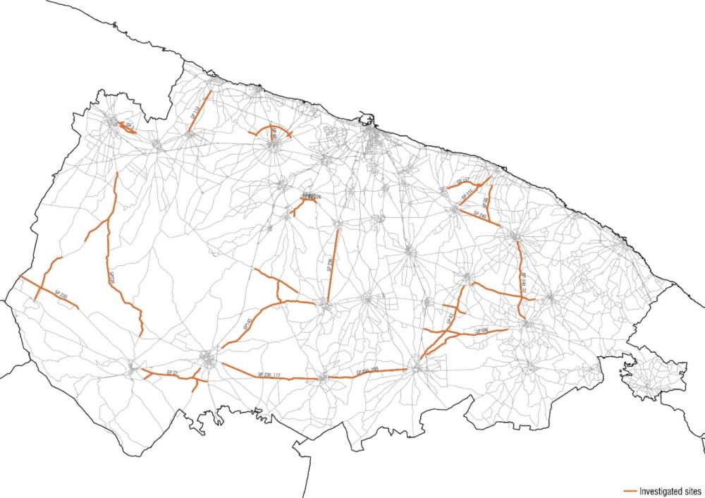
A sample of road sites was used as a testbed for the prediction of future AV scenarios, in which different traffic penetration rates are considered. In this work, 16 sites (that are small road networks, composed of individual segments and intersections) in the Province of Bari were selected. These roads are two-way, two-lane rural roads with no significant pedestrian or cyclist flows. The sites were chosen among the ones already investigated in the context of the Sustainable Urban Mobility Plans (SUMP) for the Province of Bari, based on their highlighted safety- or congestion-related issues. Hence, data about fatal and injury crashes and traffic volumes were already available. The sites are highlighted in the figure below (Figure 1).
As indicated in the introduction, exposure variables are needed in order to estimate an SPF. Moreover, other information about road site geometric configurations is preferrable. In this case, traffic volumes, total length of road sites, as well as the type and density of intersections for each road site were taken into account. Furthermore, given the specific research questions of this study, the different types and penetration of vehicles (RVs, Partially and Fully AVs) in traffic were also considered. Given that, as described in the next subsection, the definition of the crash frequency dependent variable is also based on traffic simulations, it was not possible to use a pure micro-level approach for the SPF development, in which geometric characteristics of individual segments and intersections are considered. However, the approach was also different from macro-level SPFs (see e.g., Huang et al., 2016) in which geographic, socio-economic and transport-related variables are used to predict crash frequencies in different geographic areas, possibly also considering spatial methods (Lord et al., 2021). These methodological aspects are clarified below.
2.4. Exposure variable definition
Regularly, SPFs present in their formulation (1) a coefficient dealing with the exposure of vehicles to crashes, represented by the annual average daily traffic, AADT, at the site. In this specific case, the proposal is to include in this variable not only the traditional indication about the volume (AADT) travelling on the road, but also about the market penetration of each vehicle type and its intrinsic contribution to road safety performances, given the specific aims of this study. Considering these points, this exposition variable should be defined with the twofold purpose in mind of accounting for both the traffic volume of each vehicle typology and its impact on safety. This variable is called Tr1 in the model, and it is defined as detailed below.
The market penetration stands for the quantity of vehicles of each proposed type (RVs, PAVs, FAVs) travelling on roads. The sum of the AADT of each vehicle type (RVs, PAVs, FAVs) on the road should give the total AADT travelling at the site. The AADT was then converted into an equivalent AADT. This latter variable combines a baseline traffic volume with a specific safety potential related to each vehicle type, by means of a Hazard Index (HI), a factor multiplying each vehicle type’s AADT. The HI represents the tendency of each vehicle type to be involved in a crash, determined through traffic simulations. Traffic simulations were run once each with just one vehicle category on the road network (100% FAVs; 100% PAVs; 100% RVs). In this way, each simulation provided the number of conflicts (lane-changing, crossing, rear-end) for each of the three types of vehicles (FAV, PAV, and RV). Vehicle trajectories were extracted from the simulation output. Once a surrogate safety measure had been selected, i.e., the Time To Collision (Coropulis et al., 2024), the number of conflicts was estimated. This step was run using the SSAM (Safety Surrogate Analysis Model) algorithm. Of course, the detected conflicts, as previously mentioned, are only related to multiple vehicle dynamics, excluding single-vehicle ones, even if they could represent a big portion of the possible AV conflicts. This is due to the capabilities of the SSM selected in defining conflicts and the purpose of the study, which is to investigate the impact of AVs on traffic safety. Finally, for each simulation, the number of conflicts was converted into the number of expected crashes using the Lomax Distribution (Tarko, 2018):
Where:
-
is the expected number of crashes from the conflicts detected through the SSAM across the observation period
-
k is the conversion coefficient for fatal and injury crashes (F+I). By multiplying k, the total number of crashes is converted into the number of F+I crashes. Its value for rural roads was set equal to 0.20 (Colonna et al., 2021; Vernon et al., 2004)
-
is the probability, P, of a crash, indicated as C, given the conflict, N, recorded at separation s
-
is a separation smaller than the comfortable one thus, the threshold applied to claim a conflict. The selected separation is Time To Collision (TTC)
-
is the number of traffic conflicts detected through the SSAM across the observation period based on the selected separation.
This Equation (2) contains the P(C|N, s) term that can be explained as follows: when the generic separation value for each detected conflict, sN (generic separation value obtained by the simulation for each detected conflict), is greater than a fixed threshold, s, the probability P that a conflict, N, becomes a Crash, C, is null. For all the values of sN less than the threshold, s, the probability increases from 0 to 1 depending on the recorded separation value. Thus, the outcome of Equation (2) is obtained by multiplying the calculated probability by the number of conflicts and the conversion coefficient.
The separation threshold was diversified according to the different scenarios investigated. In the scenarios including more than half of RVs and PAVs, the TTC was set equal to 1.5 s; otherwise, equal to 0.5 s (Morando et al., 2018; Papadoulis et al., 2019). This difference is justified not only by simulation outcomes (Papadoulis et al., 2019) but also by analyses of the human adaptability to AVs in a driving context. As highlighted by de Zwart et al. (2023), RVs in mixed traffic with several AVs may tend to adapt their style to that of the AVs, i.e., reducing the time headway and head distance (with AVs more than 50% of the total traffic). Wen et al. (2022) demonstrated the opposite, i.e., that in a promiscuous scenario characterized by a great variability of RVs and AVs, RVs may tend to increase their TTC, compared to their TTC against other RVs. Moreover, from investigating the California DMV (Department of Motor Vehicles) Autonomous Vehicle Collision Reports, it emerged that AVs are involved in minor but frequent collisions with RVs, due to misbehavior of RVs that do not adequately perceive the maneuvers of the Autonomous Vehicle, when stopping/slowing down, while crossing, or in parking areas. As also highlighted by previously mentioned studies, RVs seem to be more prone to reduce headway in the presence of AVs without high promiscuity. The specific analysis of interactions between Level 4 AV-RV (Morando et al., 2018) highlighted that as AV market penetration increases, road safety increases accordingly. These results from literature and crash reports are the basis for the choices made for the selection of the TTC threshold for the Lomax distribution approach. This choice implied accounting for the interactions of AVs and RVs in the definition of conflicts and then crashes.
First of all, the crashes were collected for the simplest scenarios (100% FAVs; 100% PAVs; 100% RVs), simulating 1 year. Hence, the crash frequency for each site in each of the simulated 100% scenarios was calculated according to Equation (2). The same approach was pursued for all the other scenarios proposed in Table 2, not only for the 100% ones that were propaedeutic for the HI calculation. As for the latter calculation (HI value), the crash frequency for each 100% scenario was averaged over the investigated sites. In this way, it was possible to get the riskiness associated with each type of vehicle (FAVs, PAVs, RVs). Therefore, the calibration of the HI index is derived from safety calculations. The HI index accounting for the AV penetration through the equivalent AADT (Tr1 variable) required the use of a benchmark to weigh the safety potential of the vehicle typology. Thus, the proposed HI index was calculated as follows:
Where:
-
stands for the Hazard Index related to the j-th vehicle type
-
stands for the crash frequency calculated in the scenario with 100% of the j-th vehicle type
-
stands for the crash frequency calculated in the scenario with 100% of PAVs.
According to Equation (3), it is immediately clear that three HIs needed to be calculated: one for 100% FAVs, one for 100% RVs, one for 100% PAVs (HI = 1, since the PAVs was used as the benchmark). It is evident that HI determination derived from strict calculations. Then, based on the HIs, the j-th AADT of each site was converted into the equivalent AADT for each j-th vehicle type, assigning to each vehicle category its impact on safety, multiplying by the related HI. The sum of each j-th vehicle type provided the overall equivalent AADT, i.e., Tr1.
In this way, the market penetration and the potential safety impact of vehicles were considered together by means of only one variable.
The results showed how the absence of RVs improved the safety of each site, especially if 100% of FAVs are deployed on roads. In fact, the FAVs have an HI (Hazard Index) equal to 0.76 if compared to the PAVs. The RVs have an HI of 3.59 compared to the PAVs. In this optic, the scenarios 2030, 2040, and 2050 were represented using the equivalent AADT, Tr1 (see Table 3).
| Investigated Scenarios | Calculated metric | AADT | AADT equivalent (Tr1) | ||||||
|---|---|---|---|---|---|---|---|---|---|
| FAVs | PAVs | RVs | Tot | FAVs eq | PAVs eq | RVs eq | Tot eq | ||
| 2030 | Mean Value | 0.00 | 6052.50 | 2017.63 | 8070.13 | 0.00 | 6052.50 | 7236.38 | 13288.88 |
| Standard deviation | 0.00 | 3357.29 | 1119.09 | 4476.38 | 0.00 | 3357.29 | 4013.87 | 7371.16 | |
| 2040 | Mean Value | 1614.00 | 5447.06 | 1008.75 | 8069.81 | 1222.75 | 5447.06 | 3618.13 | 10287.81 |
| Standard deviation | 895.29 | 3021.63 | 559.47 | 4476.39 | 678.29 | 3021.63 | 2006.66 | 5706.50 | |
| 2050 | Mean Value | 4841.75 | 2824.38 | 403.56 | 8069.69 | 3668.06 | 2824.38 | 1447.38 | 7939.81 |
| Standard deviation | 2685.87 | 1566.68 | 223.83 | 4476.39 | 2034.76 | 1566.68 | 802.94 | 4404.33 | |
As is blatantly obvious from Table 3, Tr1 values are averagely low, always lower than 20,000 vehicle/day except for one case.
The simulations to investigate the 2030, 2040, and 2050 scenarios, as the ones for the HI formulations, were run not focusing on single geometric elements, like intersections or segments, but on the entire site (that is a small road network), which includes several intersections and segments, in order to provide a realistic and holistic driving scenario in which vehicles have time and space to act and react to traffic variations over the sections. In this way, the recorded conflicts could have better explained the entire interaction mechanism among vehicle types.
2.5. Geometric variable definition
The other aspect to consider for prediction purposes is the road site geometry. The length of the sites and the presence of intersections have been considered. In particular, a variable counting the intersection typology (4-legged, 3-legged, and roundabout), the intersection density Ik (intersection/km), and the combination of different intersection types at each site was defined.
Similarly to the HI, a combined geometric variable was defined by assigning weights to each intersection typology based on previous safety studies. Weights are determined considering CMFs and SPFs for specific intersection types, taken from the CMF Clearinghouse[2] and the Pract-Repository[3]. As for the HI index, the calculated weights accounted for fatal and injury crashes, according to the crash typology available in the dataset used for validation and calibration of the simulation model (Coropulis et al., 2024).
The weight factor was basically a CMF (crash modification factor) assessing the different risk, in terms of crashes, between two alternatives. The CMF requires a benchmark solution to be compared to an alternative solution/countermeasure. To obtain a conversion factor, the CMF was calculated as follows:
Where:
-
represents the conversion factor of the k-th intersection typology
-
represents the crash frequency calculated for the k-th intersection typology -3-legged intersection; 4-legged intersection; roundabout-
-
represents the crash frequency calculated based on the HSM (2010) safety performance function valid for fatal and injury crashes on 3-legged intersections on two-way two-lane rural roads.
In the case of 4-legged intersections, to obtain the weight, the value in the previous equation (5) was set as the result of the application of the fatal and injury SPF taken from the HSM (2010) for two-way two-lane rural road 4-legged intersections. Whereas in the case of roundabouts, the was directly estimated based on the study made by Isebrands and Hallmark (2012) for roundabouts on rural roads, given the particular case under study. Note that other additional SPFs were developed over time for 3-/4-legged intersections (NASEM, 2021) and roundabouts (NASEM, 2019). However, the proposed references were deemed functional for the sake of simplicity and reproducibility, given their essential use for making comparisons rather than for providing precise estimates.
Thanks to equation (5), the CMF (i.e., the influence of an intersection typology compared to the 3-legged one) was obtained for each intersection of each road site. In the case of 3-legged intersections, it is always equal to 1, while for the 4-legged intersection type it depends on the specific AADT values (i.e., the application of the base intersection SPFs is dependent on traffic volumes). After these calculations, the obtained CMFs were averaged over all the road sites, resulting in an average for 4-legged intersections equal to 1.872. In the case of roundabouts, CMF = 0.13, taken from Isebrands and Hallmark (2012), is related to the conversion of 4-legged intersections (there are only two 3-legged intersection cases in the study dataset) on two-way two-lane rural roads into one-lane roundabouts. Hence, given that the reference case used in equation (5) is the 3-legged intersection, this CMF was recalibrated considering the already defined weight factor for 4-legged intersections compared to 3-legged ones. Thus, finally, the calculated used for each roundabout is equal to 0.243. Given that it is a fixed value, the average over all the corresponding sites is still equal to 0.243.
The CMFs calculated in this way were used as coefficients for considering the crash risk derived from the presence of different intersection types at the same site. Hence, these coefficients were multiplied, respectively, by the intersection density for each type of intersection (expressed in the following equation as IRoundabout; I3-Legged; I4-Legged). Then the products were summed up to obtain an indication of their combined effect on safety. The obtained variable was called Com2 since it is the combination of 2 factors regarding the intersections (density and typologies).
In this way, it was possible to consider the influence of intersections on crash occurrence (see Table 4).
| Calculated Metrics | Intersection number | Length (km) | Intersection density (Int/km) | Com2 | ||||
|---|---|---|---|---|---|---|---|---|
| 3-legged | 4-legged | Roundabout | 3-legged | 4-legged | Roundabout | |||
| Mean value | 2.18 | 1.00 | 1.25 | 14.97 | 0.12 | 0.05 | 0.07 | 0.23 |
| Standard deviation | 1.25 | 0.00 | 0.71 | 9.05 | 0.19 | 0.07 | 0.11 | 0.20 |
2.6. Statistical modeling
The SPF for AVs was estimated using a general linear model in which the error distribution follows a negative binomial structure (see e.g., Lord & Mannering, 2010). The two independent variables are Tr1 and Com 2, and the outcome, i.e., the dependent variable, is the crash frequency. The crash frequency of F+I crashes, N, is calculated as the number of crashes (obtained from simulations with mixed traffic as expressed in Table 1), per year.
The assumed SPF model equation is the following:
Where L is the total length of the i-esim road network site, and β0 (intercept), β1 and β2 are the estimated coefficients.
The goodness of fit of the model was assessed by calculating the Nagelkerke R2 as well as the residuals for obtaining the CuRe Plot, considering the independent exposure variable Tr1, instead of the usual AADT, used in previous research (Claros et al., 2018; Hauer & Bamfo, 1997; Intini et al., 2019).
The SPF was calculated for the period ranging from 2030 to 2050, to account for all the possible levels of market penetration.
2.7. Sensitivity analysis for HI influence on final safety outcome
To test the importance of the HI on the outcome of the developed SPF, a sensitivity analysis was run considering, for the same investigated years (2030, 2040, 2050), different penetration rates of FAVs, PAVs, and RVs, considering optimistic, realistic, and pessimistic projections. In this way, the Tr1 variable varied according to the different hypothesized scenarios thanks to the HI values. Intervening directly on the HI value, testing different alternatives would not have been coherent with the procedure used for the HI determination. For this reason, the sensitivity analysis was pursued, keeping the HI set to the determined values but varying the penetration rates of vehicles to allow a greater variability. The proposed penetration rates are the following (Table 5):
| Vehicles (%) | Scenarios for HI sensitivity | ||||||||
|---|---|---|---|---|---|---|---|---|---|
| Short-term (Year 2030) | Mid-term (Year 2040) | Long-term (Year 2050) | |||||||
| Pessimistic | Realistic | Optimistic | Pessimistic | Realistic | Optimistic | Pessimistic | Realistic | Optimistic | |
| RVs | 60 | 50 | 40 | 20 | 17.5 | 12.5 | 15 | 5 | 5 |
| PAVs | 40 | 50 | 60 | 67.5 | 65 | 67.5 | 55 | 60 | 50 |
| FAVs | 0 | 0 | 0 | 12.5 | 17.5 | 20 | 30 | 35 | 45 |
3. Results and Discussion
The two tested independent variables Tr1+Com2 can be both retained in the model, as based on the results shown in Table 6.
| Coefficient estimates | Std. Error | z value | Pr (>|z|) | ||
|---|---|---|---|---|---|
| Total crashes | |||||
| (Intercept) | -3.143*** | 2.898 x10⁻¹ | -10.844 | < 2 x10-16 *** | |
| Tr1 | 1.897 x10⁻⁴*** | 2.253 x10⁻⁵ | 8.418 | < 2 x10-16 *** | |
| Com2 | 2.328*** | 6.831 x10⁻¹ | 3.408 | 6.540 x10⁻⁴ *** | |
| Goodness of fit measures | |||||
| Nagelkerke R2 | 0.743 | ||||
Hence, the two independent variables chosen to depict the three different scenarios (from 2030 to 2050) and the relative difference in crash occurrence are Tr1 and Com2. They are linked according to the following equation:
As far as the goodness of fit is concerned, the Nagelkerke R2 can be considered acceptable. Thus, this developed function seems to be able to reproduce what happens with the different market penetration rates of technology. The goodness-of-fit of the model is acceptable considering that a series of subsequent approximations could have reduced the reliability of the estimates. First, the “observed crashes” for the three scenarios that constitute the baseline for the validation of the SPF derive from simulations, which are in turn affected by the parameters used to depict the different types of vehicles and their behavior. Moreover, the trajectories obtained as output from the simulations were elaborated on the basis of the Safety Surrogate Measure (SSM) chosen for the definition of conflicts. The selection of one SSM or another and its threshold may strongly affect the outcome, i.e., the number of conflicts detected in the post-processed trajectory. Additionally, the crashes are derived from the conversion of conflicts. Furthermore, the methodology used for this conversion can influence the outcome: relying on univariate or bivariate extreme value models undoubtedly affects the total number of crashes; therefore, the dataset for the development of the SPF model. Nonetheless, the goodness-of-fit of the model can be considered acceptable, considering other similar studies on traditional crashes (Giuffrè et al., 2018).
This result is the first attempt to define new SPFs in the case of AVs. This prototype seems to be valid for the proposed boundary conditions and reliable in the case of new technologies on roads, in the absence of robust datasets from the FAV and PAV crashes. Starting from the developed model (Eq. 8), it would be possible to adapt the equation, and therefore the coefficients, to several possible different scenarios since the main variables have been formulated, as well as their nature. Starting from the assumption that the two-step procedure for crash detection has already been validated (Coropulis et al., 2024), the next step can be calibrating the proposed function (Eq. 8) to other contexts and scenarios, simply varying the input data. In this way, the calibration coefficient (HSM, 2010) can be developed to extend the applicability of the proposed function. This consideration depends on the fact that the investigated sites are limited and related to an Italian case study, in which only two-way two-lane rural roads were considered. Varying one of these three starting points (geographic area, site typology, road type), the calibration can lead to different results, and the values of the parameters may consequently vary, but the function will still have the same structure.
Physically speaking, the values obtained for the developed functions show how increasing the intersections per km makes the site more dangerous; moreover, decreasing the percentage of RVs in the traffic has the opposite effect. Hence, the function represents what is supposed to happen in traffic: an increase in vehicle interactions in the presence of RVs or, at least, of humans completing driving tasks leads to a rise in dangerous situations and potential crashes. The risk related to the presence of intersections can be mitigated by the presence of FAVs rather than RVs or PAVs. By reducing both the number of intersections and the number of human-driven vehicles, the outcomes seem to be safer.
The SPF was developed on the basis of simulated crashes and not on the basis of real-world crashes since there is still a lack of data about FAV and PAV crashes, so that a robust model can be derived. In the transitory phase in which the PAVs and FAVs are not yet widely deployed on roads and there is a lack of massive datasets, it is still possible to rely on traditional SPFs for the prediction of crashes in different market penetration scenarios. This is the main contribution of the developed SPF, i.e., providing a tool for crash prediction in the absence of an observed crash dataset for AVs, but just knowing the market penetration rate of the AVs and RVs, the traffic, and the intersection characteristics and density at the site. This approach will provide preliminary safety indications, considering that the model is derived from traffic simulations. The step used to develop the presented SPF can be applied by anyone in any part of the world to calibrate ad hoc SPFs accounting for AVs, with the same approach, eventually including more variables, depending on the site conditions. The presented SPFs are valuable for depicting an ongoing scenario with different and changing penetration rates of AVs. When AVs are deployed 100% in traffic, there could be other SPFs structures or other predictive models considered reliable to depict AV behaviors and paths in traffic. In this sense, the prediction will also be corrected by weighing with observed crashes and adding all the variables and crash-leading factors. The results provided are specific to the penetration rates tested. As will be shown in the following sections, the validity range of penetration rates can affect the recalibration of the SPF coefficients. The more the traffic grows, the higher Tr1, the less precise the estimates become. This aspect is important because the SPF analyzes multiple-vehicle crashes; hence, the percentage of different types of vehicles drastically affects their interactions and the possible safety outcome.
Moreover, the results of the developed SPF can be extended to other contexts and improved once more data is available, and then more scenarios can be tested. Apart from this consideration about the value of the coefficients used to develop the SPF, the methodology and the presented variables are a solid base to rely on while considering safety assessment in the presence of AVs. It must also be considered that this SPF is the first attempt to explicitly include AVs in SPFs formulation; therefore, a simple correlation between the variables was used to introduce the problem. Of course, more complex structures can be applied in future studies, trying to diversify the impact of different vehicle types on traffic flow.
The developed SPF provides results for the three investigated scenarios based on simulated outcomes. The current unavailability of crash datasets including AVs for the investigated area, do not consent to compare the results of the SPF related to the hypothetical scenarios with observed data. Moreover, the developed SPF cannot be validated by the available observed crashes valid for RVs alone, since it is specific for AVs and can perform poorly, if applied to an RV-only scenario. Despite these limitations, the outcome of the proposed study can be useful for comparing safety outputs obtained from three different AV scenarios and, also, for thinking about possible strategies for safety improvements. This latter investigation is possible since the three scenarios have been modelled by applying the same procedure for the sake of comparability.
3.1. CuRe Plot
The goodness of fit of the model was assessed by using CuRe (Cumulative Residuals) Plots (Claros et al., 2018; Hauer & Bamfo, 1997; Intini et al., 2019) as well. The model residuals were calculated as the difference between the simulated (observed) and the predicted (by the SPF) crashes. They were arranged according to the independent variable Tr1. This variable was the most significant in the process of predicting crashes with automated vehicles, and the surrogate traffic variable is usually the one used for this kind of analysis. Then the cumulated residuals were calculated, as well as the standard deviations. All the cumulative residuals fall between the two standard deviations, showing that the variable explains the investigated phenomenon (see Figure 2).
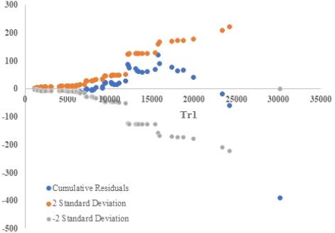
The results show that the observed crashes are greater than the predicted ones until a threshold of equivalent AADT (Tr1), equal to about 25000 vehicles/day. After this threshold, the SPF overestimates the crashes. This phenomenon is justified by the fact that the equivalent AADT increases the traffic according to the vehicle type, and due to an excess of RVs in promiscuous traffic, the hazard of the sites increases. On the contrary, when the equivalent AADT falls in the range between 10000 and 15000 vehicles/day, the simulations provide more crashes than those predicted by the model. This is because the simulations include greater traffic volumes and significantly more trajectories. More trajectories mean more potential risky situations and thus more potential conflicts. The conflicts-crashes conversion in this way overestimates the possible crashes. Therefore, the function shows some high vertical displacements in the middle ranges of Tr1.
3.2. HI sensitivity analysis
Concluding the discussion about the developed SPF, this was also verified by running a sensitivity analysis to obtain the HI impact on the overall results. Different penetration rates were hypothesized as in Table 5 to make the Tr1 vary.
In the most pessimistic scenario, the one with 60% of RVs (2030 pessimistic), the Tr1 was 2.55 times greater than the detected AADT. The results for the ratio of Tr1 over AADT for all the scenarios are summarized in Table 7.
| Scenarios for HI sensitivity | |||||||||
|---|---|---|---|---|---|---|---|---|---|
| Short-term (Year 2030) | Mid-term (Year 2040) | Long-term (Year 2050) | |||||||
| Pessimistic | Realistic | Optimistic | Pessimistic | Realistic | Optimistic | Pessimistic | Realistic | Optimistic | |
| Tr1/AADT | 2.55 | 2.30 | 2.04 | 1.49 | 1.41 | 1.28 | 1.32 | 1.05 | 1.02 |
The impact of the different penetration rates is mitigated thanks to the selected values for the HI. Of course, these results are related to mixed traffic conditions. In fact, in situations in which RVs are the only circulating vehicle type, Tr1 increases dramatically. But this side effect is contemplated by the purpose itself of the SPF, i.e., being developed and applicable for mixed traffic conditions with AVs.
In the context of this sensitivity analysis, the selected scenarios were used for calculations of the SPF outcomes. The resulting distributions of crashes are presented in Figure 3.
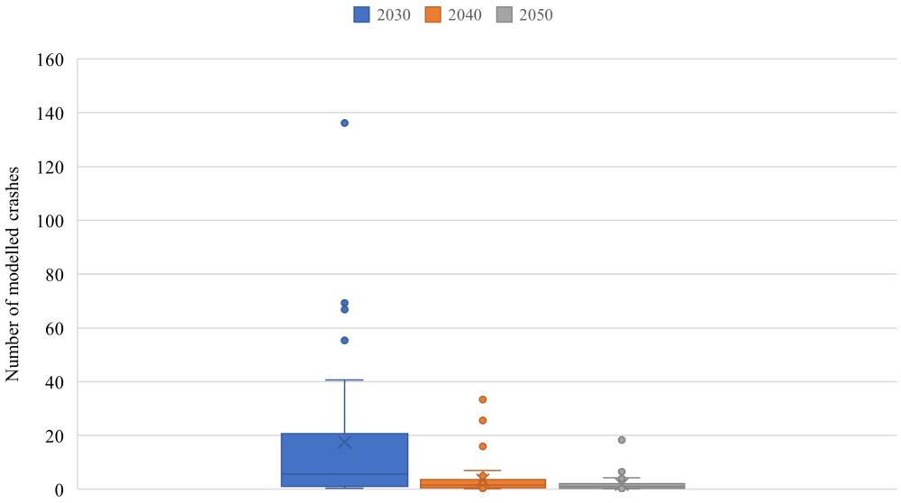
These results highlight that in the case of a higher percentage of RVs, the variance of crashes is greater than in other cases. This aspect is strictly correlated with what emerged from the CuRe Plot, i.e., great values of Tr1 (in this case affected by the preponderance of RVs) result in instability and tend to overestimate the safety outcomes. To confirm the variability induced by different percentages of vehicles and the convergence of results obtained by large percentages of AVs, the following graphs have been provided. The definition of HI has provided valuable results for the study considering the presence of AVs. Of course, for scenarios with greater values of RVs, the HI definition must be recalibrated according to the scenarios and the sites. This definition of the coefficients is strictly related to the simulated scenarios since it depends on the results of the simulations. However, the structure of the Tr1 variable as well as the entire SPF can be considered reliable for all the contexts, even if the specific coefficients might be recalibrated according to the different conditions.
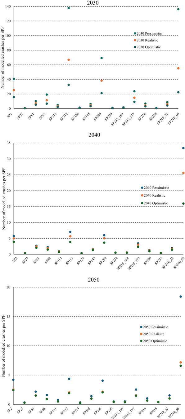
Thus, the validity range of the proposed SPF is, in this case, strictly related to the proposed scenarios (see Figure 4). For different scenarios, the SPF could necessitate parameter recalibrations. Moreover, it is obvious that RV percentages tending to 100% would make this SPF unsuitable for AV investigations. Another aspect to account for in this formulation is its validity for multivehicle crashes alone. The rationale behind this selection is that the study is based on traffic simulations, which can detect and record trajectories and elaborate on traffic conflicts happening between two vehicles. All the single vehicle crashes, including the ones due to technological failures while driving, have been neglected, because they were beyond the scope of the analysis, even if they can represent a big portion of the possible CAV (Connected and Autonomous Vehicle) accidents (Coropulis et al., 2025).
4. Conclusions
The proposed study aimed to find a new approach for determining the crash occurrence in the presence of AVs. The main focus of the research was to find a methodology that can be used in several different contexts in this infant stage of AVs on roads and that directly accounts for new kinds of vehicles in the circulating fleet and their safety impact. This aspect was crucial for the choice of the proposed methodology. In the context of safety analysis, the use of SPFs is suggested as a reliable tool for crash predictions, even if currently they have only been validated for human driving. For this reason, an ad hoc SPF was developed accounting for the presence of AVs and their interactions with other vehicle typologies, considering the transitory phase of traffic compositions. The SPF was developed for the two-lane, two-way rural roads of the Province of Bari, in the context of the SUMP analysis.
The market penetration rates of AVs are stated according to hypothetical penetration curves, for three different temporal horizons (short-term, mid-term, long-term) as stated by the SUMP.
The SPF was developed by selecting two independent variables, one related to the site geometry (intersection frequency and type, Com2) and one related to the market penetration (Tr1). The estimated coefficients associated with both variables are statistically significant at the 5% significance level. Moreover, the goodness of fit of the model was calculated by means of the Nagelkerke R2 (0.74). The goodness-of-fit shows the accuracy of the developed function for crash prediction in different scenarios. Moreover, the CuRe Plot confirms that the variable is explanatory for the investigated phenomenon.
The developed SPF can represent a powerful tool for crash prediction with AVs in the absence of observed data (which will eventually be used to recalibrate the function and to depict more complex scenarios) that could be used by decision-makers and AV manufacturers, but also by road and transport planners, calibrating it for different scenarios and contexts. Though it is true that the proposed SPF was calculated for specific boundary conditions and geographic areas, it can be used as a starting point to calibrate the coefficients of the SPF for other contexts, providing valuable results for different geometric road conditions and vehicle market penetrations. However, both its structure and reliability are affected by the fact that it has not been validated based on observed crashes, since comprehensive AV crash datasets are still lacking. Currently, there are only some crash reports developed in the USA (NHTSA Report 2021-2025 or California DVM). This aspect has been tackled by validating the simulation tool, comparing the available observed crashes with RVs with the simulated crashes in the RV-only scenario. Results from the RV-only scenario paved the way for representing the crash phenomenon by the proposed two-step methodology with simulations, in the absence of real data. The proposed SPF could not have been validated in a 100% RV scenario because it has been specifically developed for AV scenarios. Relying on traditional SPFs is highly recommended in the case of safety prediction with 0% AVs. Even if the SPF is derived from a structured procedure, the absence of a crash dataset of AVs to validate the developed SPF represents a limitation of the proposed work. Thus, this proposed SPF represents a first attempt to define a predictive method for a preliminary evaluation of AV safety, as a practical tool. It is not intended as a ready-to-use tool for making precise estimates. This is a limitation of the proposed SPF, together with the aspect that for traffic levels greater than those used for the development of the model, the SPF can lead to overestimating problems (as suggested by the CuRe Plot for Tr1 greater than 25,000 vehicles/day). The latter aspect is strictly correlated to another one, i.e., the chance of using this tool for scenarios with only RVs or high percentages of RVs. Since the proposed SPF has been developed specifically for including the AVs, its structure and its reliability are strictly connected to the presence of AVs in traffic. Thus, in the case of a great percentage of RVs in traffic (greater than 50%), the variables overestimate the traffic and consequently the crashes. Certainly, in these cases, ordinary SPFs developed for current scenarios with RVs are recommended more than the SPF developed for AVs, as in this case. Moreover, the structure of the SPF used is basic, though adequate for the study. Once a wider dataset is available and the use of AV crash data has become solid in safety analyses, more structured SPFs could be used. Another limitation of the study is the exclusion of single-vehicle crashes from analysis. These crashes represent a significant share of total crashes, and they are often associated with high-severity outcomes, but with the tool used and for the purpose of the study, they have been excluded. Since they represent a remarkable part of the road safety analysis, they should be included in further investigations based on the currently available, even if limited, observed AV crash dataset, to develop an ad hoc strategy for their quantification and mitigations.
Acknowledgement
This study was carried out within the Spoke 7 of the MOST – Sustainable Mobility National Research Center and received funding from the European Union Next-GenerationEU (PIANO NAZIONALE DI RIPRESA E RESILIENZA (PNRR) – MISSIONE 4 COMPONENTE 2, INVESTIMENTO 1.4 – D.D. 1033 17/06/2022, CN00000023). This manuscript reflects only the authors’ views and opinions. Neither the European Union nor the European Commission can be considered responsible for them.
This research was also made thanks the support of the Metropolitan City of Bari within the agreement for the “Preparation of the knowledge framework and of the ex-ante, in itinere and ex post assessment and monitoring plan of the metropolitan Sustainable Urban Mobility Plan (SUMP)”, and the Politecnico di Bari. The authors would like to acknowledge Aimsun Next for its availability in providing the traffic simulation for scientific purposes
CRediT contribution statement
Stefano Coropulis: Conceptualization, Data curation, Formal analysis, Investigation, Methodology, Resources, Software, Writing—original draft, Writing—review & editing; Nicola Berloco: Investigation, Resources, Visualization, Validation, Writing—review & editing; Paolo Intini: Data Curation, Formal analysis, Supervision, Validation, Writing—original draft, Writing—review & editing; Vittorio Ranieri: Conceptualization, Funding acquisition, Project administration, Resources, Supervision, Validation, Writing—review & editing.
Data availability
The data are available from the authors on reasonable request.
Declaration of competing interests
The authors report that they have no competing interests.
Declaration of generative AI use in writing
The authors declare that no generative AI was used in this work.
Ethics statement
This research was not subjected to ethical commission approval since it does not involve volunteers and people. However, all the research was conducted following ethical methodologies.
Funding
No external funding was used in this research.
Editorial information
Handling editor: Nicolas Saunier, Polytechnique Montreal, Canada.
Reviewers: Carmelo D'Agostino, Lund University, Sweden; Peijie Wu, Chongqing Jiaotong University, China; Mariano Pernetti, University of Campania, Italy.
Submitted: 6 October 2024; Accepted: 14 October 2025; Published: 2 November 2025.
SAE stands for Society of Automotive Engineers ↩︎
https://www.cmfclearinghouse.org/ Last access on September 30th, 2024. ↩︎
https://www.pract-repository.eu/ Last access on September 30th, 2024. ↩︎