A comprehensive approach to evaluation of road safety policy

Introduction

There is a great interest in evaluating the effects of road safety policy. Policy makers in all countries want to know how effective their policy is and how it can be made more effective. There is also an interest in learning what the contribution of road safety policy has been to the decline in the number of traffic fatalities seen in many highly motorised countries after about 1970.

Unfortunately, a rigorous scientific evaluation of the effects of road safety policy is very difficult. The difficulties include:

1. Very many factors influence road safety and reliable data are available only for a few of them. As an example, data on drinking-and-driving in Norway are only available for 1981, 2006, 2009 and 2017. Speed data are available after 2006, but only sporadically before that year.

2. The factors for which data are available tend to be highly correlated with each other and with time. This makes it very difficult to estimate their relationship to traffic fatalities precisely.

3. It is difficult to describe road safety policy adequately. It consists of long-term ideals for safety (like Vision Zero), quantified targets and a large number of road safety measures. Detailed data on the implementation of road safety measures are often lacking. Thus, the number of roundabouts in Norway is only known for 1980, 1984, 1995, 2005, 2011, and 2015.

4. There is no comparison group. While comparisons between countries have been used in studies evaluating road safety targets (Allsop et al., 2011), it is difficult to find two countries that differ with respect to road safety policy but are otherwise similar in terms of factors influencing road safety. Moreover, good data on the road safety policies pursued in different countries are hard to find.

5. The reporting of traffic injury in official statistics is incomplete and studies indicate that it has declined over time (Bø, 1970; Hagen, 1993; Lereim, 1984; Lund, 2019). Only the number of traffic fatalities is believed to be completely, or nearly completely reported in highly motorised countries.

(Elvik & Høye, 2022) discuss the use of multivariate statistical analyses to evaluate the effects of road safety policy and conclude that any such analyses are likely to be affected both by omitted variable bias and by collinearity. This refers to points 1 and 2 above. Yet, the problem is multivariate and attempts to evaluate road safety policy by means of multivariate analyses should not be abandoned unless all such analyses can be shown to be meaningless.

Elvik (2024) discusses how best to describe road safety policy, preferably in numerical terms. He proposed a road safety policy index consisting of ten items. These ten items by no means include all road safety measures that were implemented in the period covered by the study; it is simply those for which data happen to be available. No minor improvements, like guard rails, building roundabouts or installing road lighting were included. On the other hand, the use of many road safety measures is highly correlated and including very highly correlated items in an index may be redundant and amount to double counting.

Since every country has a unique road safety policy, analyses generally use annual data for a single country as the unit of observation, although some studies (Fridstrøm, 1999) have used monthly data for the counties of a country. Usually, however, annual data for a whole country are more easily available than data at lower levels of aggregation. An effect of something, like road safety policy, can be defined as changes produced by the policy that would not otherwise have happened. But how can the counterfactual, i.e. what would otherwise have happened be defined in a multivariate analysis? Elvik and Nævestad (2023) suggest one possibility, but relying on it only produces what may be termed a ʻhypotheticalʼ counterfactual, not an actual one, like in a randomised controlled trial.

This paper will try to discuss all the problems of evaluating road safety policy and indicate solutions to them. It is recognised that ideal solutions cannot be found. The paper therefore focuses on the need for exploratory analyses to support the formulation of hypotheses about the effects of road safety policy and on the need for explicitly justifying all analytic choices made with respect to, for example, the definition of variables and which variables to include in multivariate analyses. The following stages have been identified in an evaluation of road safety policy:

1. Description of trends in road safety

2. Identification of variables describing policy

3. Identification of confounding variables

4. Exploratory model development

5. Comparison of statistical models for analysis

6. Estimation of policy effect and its uncertainty.

Describing trends

The main reason for starting by describing trends over time is to get ideas for hypotheses about the effects of road safety policy. Data for Sweden for 1968–2022 will be used to illustrate this step of analysis.

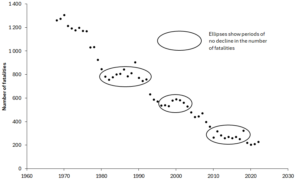
Figure 1 shows the number of traffic fatalities in Sweden from 1968 to 2022. 1968 was the first full year after the change to driving on the right. There is a clear downward trend. In 1970, there were 1307 fatalities. In 2020, the number had been reduced to 204, a reduction 84.4%. The downward trend has, however, been quite irregular. There have been periods in which there was no decline in the number of fatalities. These periods are indicated by ellipses in Figure 1. In the periods when there was decline, the rate of decline varied. There was a very sharp decline in the last half of the 1970s. In more recent times, the decline appears to be less sharp, but in percentage terms this may not be the case.

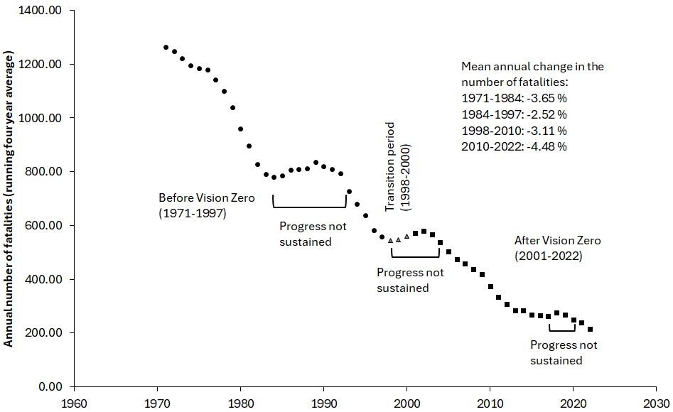
To reduce the contribution of random variation, four year running averages were computed. The first is the average of 1968, 1969, 1970 and 1971 and is denoted as 1971 in Figure 2. It is seen that the data points scatter less widely, but the periods of stagnating decline can still be clearly identified. The periods of stagnation have been labelled as ʻprogress not sustainedʼ. Each period starts when a declining trend stopped and ends the first year when the number of fatalities was lower than in the first year of the period of stagnation. Thus in 1985 the four-year average number of fatalities was higher than in 1984 (786.5 versus 780.5). The number did not go below 780.5 until 1993, when it was 727. This marked the end of the period of stagnation. However, the turning point indicating that the period of stagnation was coming to an end started earlier. The four-year average number of fatalities was lower in 1990 than in 1989 and the decline continued until 1998.

Three main periods have been identified in Figure 2: before Vision Zero, a transition period, and after Vision Zero. Vision Zero was adopted in October 1997, and the year 1997 is classified as before Vision Zero. 1998 is the first year in the after Vision Zero period.

The transition period comprises all four-year periods that include the year 1998. The mean annual change in the number of fatalities has been estimated for four periods: 1971–1984, 1984–1997, 1998–2010 and 2010–2022. The first two of these periods were before the adoption of Vision Zero, the last two after. It is seen that there was decline in the number of fatalities in all four periods. The decline was slower in 1984–1997 than in 1971–1984. The mean annual decline was 3.65% in 1971–1984. This was reduced to 2.52% during 1984–1997. In the first period after Vision Zero, annual mean decline in the number of fatalities increased again to 3.11%. It further increased to 4.48% in the most recent period.

If this variation can be linked a corresponding variation in the effects of road safety policy, this will strengthen a claim that road safety policy may explain variation in the rate of decline in traffic fatalities in Sweden. Finding such a dose-response pattern is often regarded as an indication, although by itself not a proof, of a causal relationship. This supports the following hypotheses:

• H1: Road safety policy in Sweden became more effective after the adoption of Vision Zero than it was before the adoption of Vision Zero

• H2: Road safety policy has gradually become more effective in the period after the adoption of Vision Zero. It was least effective immediately after the adoption of Vision Zero and became more effective until about 2015. After that it became less effective.

A road safety policy can become more effective by using more effective road safety measures, or by increasing the use of effective road safety measures. To believe that road safety policy can be effective, it must be shown that it consists of road safety measures that are known to be effective.

To test these hypotheses, it is necessary to describe road safety policy in numerical terms in order to determine how it has varied over time. Such a description of road safety policy requires data about the use of effective road safety measures on an annual basis. There should be no gaps in the data, and they should ideally include as many road safety measures as possible. Hypotheses 1 and 2 are supported if data show that road safety policy became more effective after the adoption of Vision Zero than it was before the adoption of Vision Zero.

Variables describing road safety policy

In general, very limited data are available on variables describing road safety policy. This applies especially to detailed data about road user behaviour. For Sweden, complete data for 1981–2018 have been found for the length of motorways and 2+1 roads with a median barrier and for the number of random breath tests. Figure 3 shows the length of motorways and 2+1 roads in Sweden from 1981 to 2018. It is seen that the length has grown more rapidly after about 2000 than before that year.

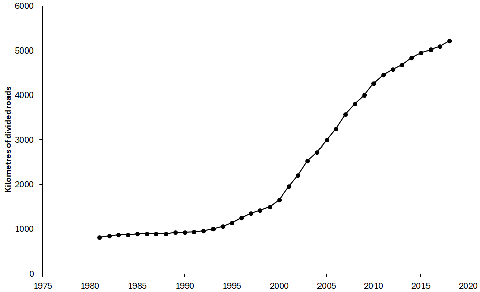
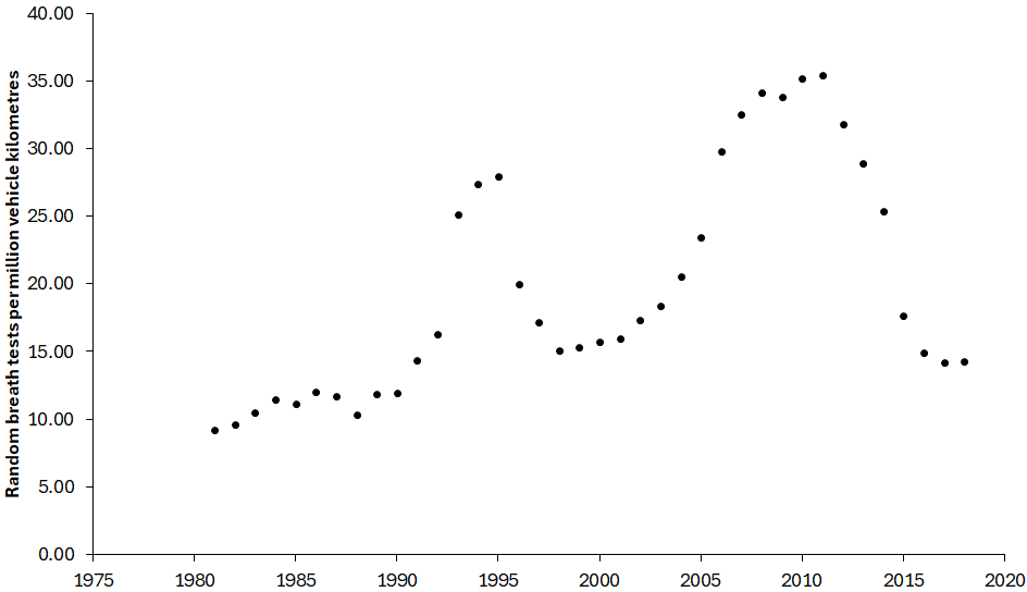
Figure 4 shows the number of random breath tests per million vehicle kilometers of travel from 1981 to 2018. The number of breath tests per million vehicle kilometers of travel changes in a wavelike pattern. There was an increase until about 1995, then a decline until about 2000. Then there was an increase again until about 2010, followed by a decline. A similar cyclical pattern has been found for citations for traffic offenses per million vehicle kilometers of travel in Norway (Elvik & Nævestad, 2023).

Both these variables are numerical and continuous and change values from year to year. This makes them suitable for inclusion in a multivariate statistical analysis. However, they do not fully describe road safety policy. Road safety policy consists of many other road safety measures in addition to these two. Moreover, the long-term ideals, principles and targets of road safety policy have changed over time. The most important change was the adoption of Vision Zero in late 1997. Another change was the adoption of a quantified target for reducing the number of traffic fatalities. A target was set in 1996 of reducing the number of fatalities from 540 in 1994 to 270 in 2007. After 2007, a new target of 220 fatalities was set for 2020.

Vision Zero can be represented as a dummy variable, taking the value of 0 for 1981–1997 and 1 for 1998–2018. The quantified targets for 2007 and 2020 are included in the form of the mean annual percentage reduction of the number of fatalities aimed for: 5.6% per year for the first target (1996–2007) and 5.2% per year for the second target (2008–2020). The targeted reduction is stated as a positive number. Hence, the following four variables describe road safety policy:

1. Length in kilometers of motorways and 2+1 roads with a median barrier

2. Number of random breath tests per million vehicle kilometers of travel

3. Dummy for Vision Zero

4. Targeted annual percentage reduction in the number of fatalities.

Confounding variables

The number of traffic fatalities is influenced by very many variables and road safety policy may not be the most important (Fridstrøm, 1999). In any analysis of road safety policy, one should try to control for as many confounding variables as possible.

In this study, a year is the unit of observation. There are 38 years in total. The number of variables that can be included in a study with such a small sample is very limited. Based on previous research (Brüde, 1995; Elvik, 2019; Wegman et al., 2017), the following confounding variables have been included:

1. Time (as a year count, with 1981 = 1 and 2018 = 38

2. Million vehicle kilometers of travel

3. Unemployment (percent of labour force; annual mean values.

Table 1 lists the data for all variables included in the study. The next stage of the study is an exploratory analysis for the purpose of developing the best model for estimating the effects of the policy variables and the confounding variables.

Exploratory model development

The variables of principal interest in the study are the policy variables. The first model developed therefore included only these variables. The results are reported in Table 2.

All models were fitted by means of negative binomial regression. As part of the comparative analysis of different statistical models, the negative binomial regression models will later be compared to a multivariate time-series model and a linear regression model based on annual differences in the value of the variables listed in Table 1.

Model 1 included only motorway kilometers and random breath tests. As expected, both variables had a negative coefficient, which was statistically significant for both variables. In model 2, Vision Zero and the quantified road safety target were added. All variables were expected to have negative coefficients, but Vision Zero did not. All coefficients were statistically significant at 5% level of significance.

To assess how robust estimated coefficients are with respect to the variables included in the models, attenuation and change of sign were estimated. Attenuation refers to a change in the estimated value of a coefficient. Thus, the coefficient for motorway kilometers was reduced from -0.0002186 in model 1 to -0.0002118 in model 2. This is a reduction of 3.1%. The coefficient was negative in both models; hence, the sign did not change.

The purpose of comparing models including different variables is to assess how stable the coefficients for the policy variables are across different models. A lack of stability, either in terms of large changes in the value of coefficients, change in the sign of coefficients, or change the precision of coefficient estimates suggest that the variables cannot be given a causal interpretation (Hauer, 2010). Only policy variables that remain stable across model specification will be included in the final model.

Models 1 and 2 did not include any confounding variables. In model 3, year was included. This was associated with a further attenuation in the coefficients for the policy variables, except for Vision Zero. Attenuation is always assessed by comparing the estimated coefficient in model n with the estimated coefficient in the first model including a variable. The rather large attenuation of the coefficients for the policy variables show that they are not robust with respect to control for confounding variables, i.e. the ‘crudeʼ coefficients estimated for these variables in the models not including any confounding variables overestimate the effects of the policy variables.

Model 4 includes all confounding variables and all policy variables. Two of the policy variables change sign from negative to positive: random breath testing and quantified target. For three of the policy variables, the coefficient is no longer statistically significant. It remains significant for motorway kilometers. In model 5, two of the policy variables were omitted. The coefficient for motorway kilometers remains negative. The coefficient for random breath testing is positive, which is implausible. However, the coefficient is far from statistical significance.

Model 6 is the final model. It includes three confounding variables and just one policy variable, motorway kilometers. The other three policy variables were not included as no reliable estimates of their effects were found in the exploratory analysis. The coefficients either changed sign in different models and/or were not statistically significant. This instability suggests that the variables cannot be interpreted as causal factors (Hauer, 2010). As can be seen by comparing the Elvik index of goodness of fit, the loss of explanatory value by omitting three of the variables included in model 4 is minimal. Model 4 explained 97.18% of the systematic variation in the number of killed road users; model 6 explained 96.97% of the systematic variation in the number of killed road users. The loss of explanatory value is only 0.19%.

Comparative analysis of statistical models

As noted above, several statistical techniques can be used to analyse data for the purpose of estimating the contribution of road safety policy to changes in the number of traffic fatalities. It is good practice to employ more than one technique of analysis and to compare the results obtained using different techniques of analysis. A general problem in the analysis of time series data, is that the variables tend to be highly correlated. Table 3 shows the correlations between the variables.

It is seen that when annual values are used for all variables, the correlations between them are very high. If variables are redefined as annual differences, e.g. rather than entering the number of killed road users as 784 in 1981 and 758 in 1982, it is entered as -26 in 1982, the correlations become much weaker, as shown in panel B of Table 3.

Three models of analysis have been compared:

1. Negative binomial regression model (model 6) in Table 2

2. A multivariate ARIMA time series model, including the same variables as the negative binomial regression model

3. A least squares linear regression model based on annual differences in the values of the variables, including the same variables as models 1 and 2.

The performance of the models is compared in terms of the following statistics:

1. Sign and statistical significance of coefficients

2. Bias in predicted values

3. Overall goodness of fit

4. Mean absolute percentage prediction error

5. Autocorrelation of residual terms

6. Cumulative residuals plot.

There has been a decline over time in the number of traffic fatalities. Based on previous studies (Elvik, 2019) the following signs are expected for the coefficients: year count: negative; vehicle kilometers of travel: positive; unemployment: negative; motorway kilometers: negative.

If model predictions are unbiased, the sum of predicted values should equal the sum of recorded values. The sum of fatalities for 1981–2018 in Sweden was 20 584. Overall goodness-of-fit is estimated by means of the Elvik index for the negative binomial regression model and by means of the squared multiple correlation coefficient (R ²) for the linear regression model. For the time-series model, a modified version of the Elvik index is used as measure of goodness-of-fit. The mean absolute percentage prediction error is the mean value of percentage prediction errors, when all these errors are entered as a positive number. Autocorrelation of residual terms is assessed at lag one, i.e. by correlating residuals at lag zero with those at lag one. Two data points (the first and last) are lost when estimating autocorrelation at lag one. Finally, cumulative residual plots (Hauer & Bamfo, 1997) have been developed to compare the models.

Table 4 summarises the comparison of the models. The estimates based on the negative binomial regression model and the multivariate time-series model are very similar. However, the time-series model fits the data better and has no autocorrelation of the residual terms. Cumulative residual plots for the two models are shown in Figure 5.

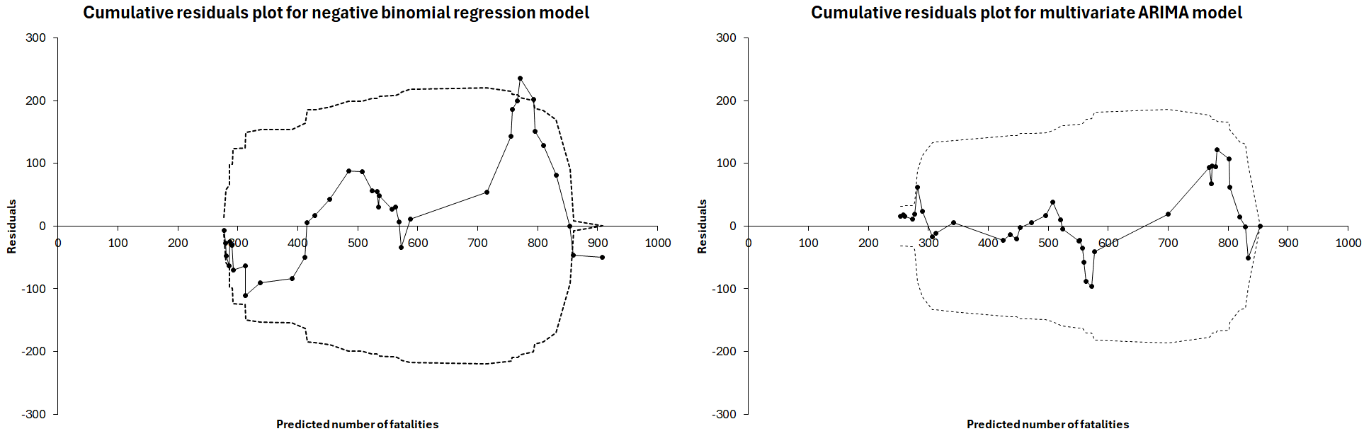
It is seen that the cureplot for the time-series model displays less variation than the cureplot for the negative binomial regression model. It strays outside the dotted line indicating plus or minus two standard errors, whereas the plot for the time-series model always stays within plus or minus two standard errors.

As far as the model based on annual differences is concerned, the results made no sense. Only one of four coefficients was statistically significant, and the entire cureplot was located outside the dashed lines indicating two standard errors. The model explained only 31.7% of the variance. The clear conclusion from the comparison of models is that the time-series model is the best model.

Estimating the effect of road safety policy

There are two equivalent ways of estimating the effect of road safety policy on the number of killed road users in Sweden during 1981–2018. The first method is to estimate a hypothetical, counterfactual number of killed road users by omitting the policy variable (motorway kilometers) from the predictive equation but keeping the other variables with unchanged (compared to the full model) values of the coefficients. The second method is to directly estimate the effect of the policy variable by multiplying the coefficient with the value of the variable each year. These two methods produce identical results.

Based on the time-series model, the number of traffic fatalities in Sweden in 2018 was 27.6% lower than it would have been without the growth in motorways and 2+1 roads. Obviously, this is an imperfect indicator for road safety policy, and it is very likely that part of the effect of road safety policy is captured by the trend term (year count). This will probably include the effects of cars becoming gradually safer. However, renewal of the car fleet is a slow process, and it takes place at a rather constant rate. This means that it is almost perfectly correlated with time and therefore difficult to estimate reliably.

Uncertainty of policy effect

The estimated contribution of road safety policy to reducing the number of killed road users in Sweden is highly uncertain. Uncertainty can be estimated by applying the lower and upper 95% confidence limit values of the coefficient for the policy variable. For the final year of the study, it is then found that:

The best estimate of the effect of policy is a reduction of the number killed road users of 27.6%. The lower 95% confidence limit is a reduction of 54.2% and the upper 95% confidence limit is an increase of 72.1%. Thus, the estimated reduction is not statistically significant. It is nevertheless far more likely that road safety policy has contributed to reducing the number of fatalities than that it has not contributed to this. This can be seen from Figure 6.

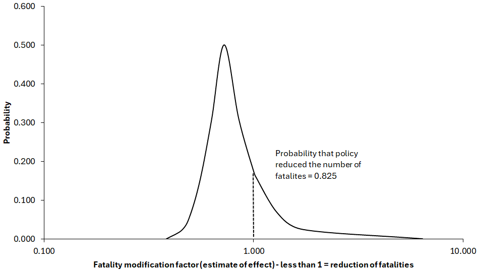
The probability that policy has reduced the number of fatalities is 0.825; the probability that it has not is 0.175. It may be noted that the negative binomial regression model produced larger estimates of policy effect. The best estimate for the year 2018 is a 42.1% reduction of fatalities, with a 95% confidence interval from 61.5% reduction to 12.9% reduction.

With respect to the hypotheses proposed in section 2, the following results were obtained from the time-series model: The simple mean annual reduction of fatalities, attributed to the policy indicator, during 1981–1997 was 0.2%. During 1998–2018, it was 1.3%. This supports hypothesis 1. The period after Vision Zero has been divided into 1998–2004, 2005–2014 and 2015–2018.

During 1998–2004, road safety policy contributed to a mean annual decline in fatalities of 0.8%. This increased to 2.2% during 2005–2014, but slowed down to a complete halt during 2015–2018, with an estimated annual increase of 0.2% in the number of fatalities. This pattern supports hypothesis 2.

Discussion

A rigorous evaluation of the effects of road safety policy is impossible, and the analyses reported in this paper confirm this. Two main difficulties continue to resist a good solution. These are:

1. It is not possible to define a variable, or set of variables, which adequately describes road safety policy.

2. Any variable, or set of variables, describing road safety policy is very highly correlated with time and with other slowly changing variables, like vehicle kilometers of travel.

In an ideal world, there would be a complete historical record of when all road safety measures were implemented. It would be possible to reconstruct, for example, exactly how many roundabouts were built each year in Sweden after 1981 and the traffic volume in these roundabouts. In theory, these data may exist in the national road data bank, but most likely not in an easily readable form. One would have to identify each roundabout and record the data for it in a separate file. However, there would almost certainly be gaps in the data. Some roundabouts would not have data about construction year. Some would not have complete data on traffic volume. Some would have been modified one or more times after initial construction.

Besides, even in the unlikely case that the road data bank is complete and has no erroneous or missing information, it is not a statistical database that easily lends itself to tabulating the data in summary form, i.e. as total, annual numbers for of all of Sweden. Moreover, somewhat arbitrary decisions would have to be made with respect to what to include and count as road safety measures. Should, for example, resurfacing of roads, provided data existed about it, be included? Should replacing worn traffic signs be included? Or are these measures too trivial to be included?

Reconstructing historically the implementation of all road safety measures would be draconian task if the data existed. However, the data do not exist, and we are thus spared from the draconian task. Long time series of data exist only for very few road safety measures. In Sweden this includes the length of motorways and 2+1 roads, the number of random breath tests, the number of speed cameras, and seat belt wearing. Major changes in speed limits may also be reconstructed. The dates of important new legislation, like mandatory daytime running lights, are known. Apart from this, we essentially know nothing about the history of road safety measures and hence nothing about the history of road safety policy.

Yet, even if we try to include and code as numerical variables what little we do know, these variables will be highly correlated with other variables we want to include—various confounding variables we want to control for. Four variables describing road safety policy were tested in this study. Only one of them was found to have a statistically consistent relationship to the number of fatalities: the length of motorways and 2+1 roads. The other three variables either switched sign depending on which other variables were included in the models or became statistically insignificant. This lack of consistency does not support a causal interpretation of these variables. Besides, with data for only 38 years, it is not possible to include more than about 4 independent variables in a statistical analysis.

The final models included just four independent variables, but these were highly correlated. The multivariate time-series model was clearly the best of the three statistical models that were compared. The estimate of the effect of road safety policy in 2018 based on this model, a fatality reduction of 27.6% is implausibly low. A trend line fitted to the number of fatalities from 1981 to 2018 shows a total reduction of 72.6%. If the estimated contribution from policy is correct, it explains only 38% of the decline. This is probably too low, and contributions from, for example, safer cars are embedded in the trend term (the year count variable). In short, the main result of the study is probably misleading and nothing can be learned from it with respect to future development of a more effective road safety policy. We are, in other words, not in a position where we can learn anything from the history of road safety policy, at least not based on the approach adopted in this paper.

As a sensitivity analysis, a simple policy index was developed by adding the values of motorway length and random breath tests per million vehicle kilometers of travel. The value of the index was set equal to 100 for 1981. It grew irregularly, reaching a maximum value of 465 in 2011, then declining to 387 in 2016, before increasing again to 395 in 2018. The results of a time-series analysis using this index were similar to those obtained using only motorway length. Road safety policy became more effective after adopting Vision Zero and was at its most effective until about 2011.

One possible approach to strengthen the basis for causal inferences would be to do separate analyses for rural and urban areas. One would then expect, for example, the contribution of motorways to reducing fatalities to be larger in rural areas than in urban areas. Such a finding would support what Fridstrøm (2015) calls the ‘casualty subset testʼ: A road safety measure should have a larger effect within a clearly designated target group than outside the target group. On the other hand, it might be the case that fatalities have been reduced just as much, or more, in urban areas than in rural areas—not as a result of new motorways, but perhaps as a result of traffic calming and more roundabouts. However, as long as the available data on traffic calming and roundabouts are too incomplete to include in a statistical analysis, the decline would, erroneously, be attributed to new motorways. Even more absurd examples can easily be found. In one model developed for Norway (unpublished, as part of exploratory analysis), increased seat belt wearing was found to be associated with fewer pedestrian and cyclist fatalities. The two variables simply happened to be highly correlated in time, but there clearly is no causal relationship between them.

It may perhaps be more fruitful to combine a detailed study of trends, and shifts in them, with historical data on specific decisions and implementation of specific road safety measures. The trends shown in Figure 2 clearly show that there have been periods both of fast and slow decline in the number of fatalities, as well periods of increase. Can these variations be linked to changes in road safety policy? In answering this question, a statistical analysis based on a single variable indicating road safety policy will be inadequate and not capture the dynamics of policy. It is, for example, interesting to note that Vision Zero was adopted during a period when the decline in the number of fatalities appeared to have stopped. Vision Zero quickly gained broad political support as an attractive idea and renewed political interest in road safety. Changes like this are difficult to capture in a statistical model. Yet, it did take some years before a rapid decline in the number of traffic fatalities in Sweden started. Clearly, part of the large declines in 2008, 2009 and 2010 were caused by the economic recession in those years. But 2008 was the year when speed limits were lowered on many roads in Sweden. An evaluation (Vadeby & Forsman, 2018) estimated that the changes in speed limits reduced the number of fatalities by 17 per year.

Thus, a hybrid analysis, a mixture of a detailed examination trends and changes in them, combined with data about specific policy decisions may perhaps be the most informative approach for evaluating the effects of road safety policy.

Conclusions

The main conclusions of the study presented in this paper can be summarised as follows:

1. A time-series analysis indicates that in 2018, the number of traffic fatalities in Sweden was about 28% lower than it would have been if no road safety policy had been implemented.

2. Road safety policy is indicated by a single variable, the length of motorways and 2+1 roads. This indicator is likely not to capture all effects of road safety policy.

3. The true effect of road safety measures implemented during 1981–2018 is most likely greater than indicated by the analysis reported in this paper.

Declaration of competing interests

The author declares that he has no competing interests.

Funding

This research was funded by the Swedish Transport Administration, grant 5448.

CRediT contribution statement